教程3：Cell Classification（细胞分类）

目标：展示如何基于 GridScore 与放电率统计进行细胞分类，并输出分类结果与可视化。

结构：

1. 任务概览

2. 计算 GridScore

3. 分类方法示例

4. 输出与可视化

Note

本教程以 examples/cell_classification 中脚本为参考，偏重示例与流程。 若需要完整 ASA pipeline，请先阅读 教程1：ASA Pipeline：实验数据解码全流程。

0. 任务概览

细胞分类通常基于以下信息：

• GridScore：衡量放电场是否呈网格结构

• 放电率与空间选择性：用于筛选候选细胞

• 模块划分：通过自相关特征聚类识别不同网格模块

本教程展示两条实践路径：

1. 单细胞 GridScore 评分与可视化

2. 基于自相关特征的模块识别（分类）

1. 计算 GridScore

示例脚本：examples/cell_classification/grid_score.py

关键步骤：

• embed_spike_trains 将 spike 事件嵌入为 (T, N) 矩阵

• compute_rate_map_from_binned 生成 rate map

• compute_2d_autocorrelation 计算自相关

• GridnessAnalyzer.compute_gridness_score 得到 GridScore

from canns.analyzer import data
from canns.analyzer.data.cell_classification import (
    GridnessAnalyzer,
    compute_2d_autocorrelation,
    compute_rate_map_from_binned,
    plot_autocorrelogram,
    plot_rate_map,
)
from canns.data.loaders import load_grid_data, load_left_right_npz

grid_data = load_grid_data()
cfg = data.SpikeEmbeddingConfig(smooth=False, speed_filter=True, min_speed=0.0)
spikes, xx, yy, _tt = data.embed_spike_trains(grid_data, config=cfg)

analyzer = GridnessAnalyzer()

neuron_id = 69
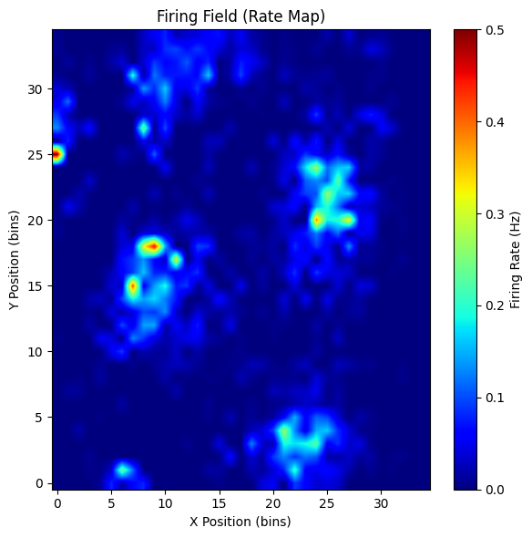
rate_map, *_ = compute_rate_map_from_binned(xx, yy, spikes[:, neuron_id], bins=35)
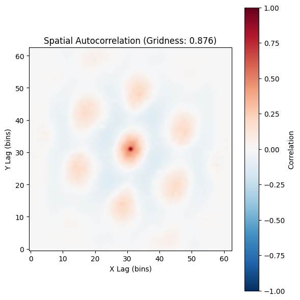
autocorr = compute_2d_autocorrelation(rate_map)
result = analyzer.compute_gridness_score(autocorr)
print(f"neuron {neuron_id}\nscore: {result.score}\nspacing: {result.spacing}\norientation: {result.orientation}")

# Visualize rate map + autocorrelogram
plot_rate_map(rate_map, show=True)
plot_autocorrelogram(autocorr, gridness_score=result.score, show=True)

Loaded grid_1: 172 neurons
Position data available: 238700 time points
neuron 69
score: 0.8761650577011183
spacing: [18.43908891 17.08800749 18.11077028]
orientation: [-40.60129465  20.55604522  83.65980825]

(<Figure size 600x600 with 2 Axes>,
 <Axes: title={'center': 'Spatial Autocorrelation (Gridness: 0.876)'}, xlabel='X Lag (bins)', ylabel='Y Lag (bins)'>)

2. 分类方法示例

示例脚本：examples/cell_classification/try_classification_methods.py

该示例使用自相关图作为特征，采用 Leiden 聚类识别网格模块。 核心函数：

• identify_grid_modules_and_stats：输出模块划分与统计信息

from canns.analyzer.data.cell_classification import (
    GridnessAnalyzer,
    identify_grid_modules_and_stats,
    compute_rate_map_from_binned,
    compute_2d_autocorrelation,
)
import numpy as np

grid_data = load_left_right_npz(
    session_id="28304_1",
    filename="28304_1_ASA_mec_full_cm.npz",
)
n_units = spikes.shape[1]
autocorrs = []
for nid in range(n_units):
    rate_map, *_ = compute_rate_map_from_binned(xx, yy, spikes[:, nid], bins=35)
    autocorr = compute_2d_autocorrelation(rate_map)
    autocorrs.append(autocorr.astype(np.float32, copy=False))

autocorrs = np.stack(autocorrs, axis=0)

analyzer = GridnessAnalyzer()
out = identify_grid_modules_and_stats(
    autocorrs,
    gridness_analyzer=analyzer,
    k=30,
    resolution=1.0,
    score_thr=0.3,
    consistency_thr=0.5,
    min_cells=10,
    merge_corr_thr=0.7,
    metric='manhattan',
)
print(out['n_grid_cells'], out['n_modules'])

106 1

/Users/sichaohe/Documents/GitHub/canns/src/canns/analyzer/data/cell_classification/utils/image_processing.py:284: FutureWarning: `binary_dilation` is deprecated since version 0.26 and will be removed in version 0.28. Use `skimage.morphology.dilation` instead. Note the lack of mirroring for non-symmetric footprints (see docstring notes).
  dilated = morphology.binary_dilation(image, footprint=footprint)

3. 输出与可视化

• grid_score.py 会绘制 rate map、自相关图与 GridScore 直方图

• try_classification_methods.py 会保存 grid_modules_demo_output.npz

建议：

• 先用小批量神经元验证参数，再扩大到全体

• 适当调整 bins / score_thr / consistency_thr 以匹配数据质量

• 若需与 ASA pipeline 联动，可将 spikes 与 x/y/t 与解码结果结合分析