How to Train Brain-Inspired Models?

Goal: By the end of this guide, you’ll be able to train a Hopfield network to store and recall patterns using Hebbian learning.

Estimated Reading Time: 12 minutes

Introduction

Unlike deep learning models trained with backpropagation, brain-inspired models use biologically plausible learning rules like Hebbian learning [22].

This guide introduces:

1. The Hebbian learning principle

2. Training a Hopfield network for pattern memory

3. Using the Trainer framework

4. Key differences from deep learning

We’ll train a model to memorize and recall images—demonstrating associative memory in action.

What is Hebbian Learning?

Hebbian learning [22] is an unsupervised learning rule where synaptic weights strengthen when pre- and post-synaptic neurons are co-active:

Δw_ij = η × x_i × x_j

Where:

• w_ij: Connection weight from neuron i to neuron j

• x_i, x_j: Activities of neurons i and j

• η: Learning rate (often set to 1 for simple rules)

Key properties:

• Local: Weight updates depend only on activities of connected neurons (no global error signal)

• Unsupervised: No labels or target outputs required

• Biologically plausible: Matches synaptic plasticity observed in real neurons

Contrast with backpropagation:

• Backprop: Global error signal, supervised, requires differentiable loss

• Hebbian: Local activity, unsupervised, no gradient computation

Amari-Hopfield Network

An Amari-Hopfield Network [21, 23] is a recurrent network that stores patterns as stable attractor states. When presented with a partial or noisy pattern, the network converges to the nearest stored memory.

Use case: Associative memory, pattern completion, error correction

from canns.models.brain_inspired import AmariHopfieldNetwork  # :cite:p:`amari1977neural,hopfield1982neural`

# Create a Hopfield network with 16,384 neurons (128x128 flattened image)
model = AmariHopfieldNetwork(
    num_neurons=128 * 128,  # Image size when flattened
    asyn=False,             # Synchronous updates (all neurons update together)
    activation="sign"       # Binary activation: +1 or -1
)

Parameters:

• num_neurons: Network size (must match input dimensionality)

• asyn: Asynchronous (one neuron at a time) vs synchronous updates

• activation: “sign” for binary Hopfield, “tanh” for continuous variant

The Trainer Framework

The library provides a unified Trainer API that abstracts training logic:

Model + Trainer + Data → Trained Model

Philosophy (from the Design Philosophy docs):

• Separation of concerns: Model defines dynamics, Trainer defines learning

• Reusability: Same trainer works for different models with compatible learning rules

• Composability: Stack trainers for multi-stage training

For Hebbian learning, we use HebbianTrainer:

from canns.trainer import HebbianTrainer

trainer = HebbianTrainer(model)

Key methods:

• trainer.train(data): Train on a list of patterns

• trainer.predict(pattern): Recall a single pattern

• trainer.predict_batch(patterns): Batch recall (compiled for speed)

Complete Example: Image Memory

Let’s train a Hopfield network [21] to memorize 4 images and recall them from corrupted versions.

Step 1: Prepare Training Data

import numpy as np
import skimage.data
from skimage.color import rgb2gray
from skimage.transform import resize
from skimage.filters import threshold_mean

def preprocess_image(img, size=128):
    """Convert image to binary {-1, +1} pattern."""
    # Convert to grayscale if needed
    if img.ndim == 3:
        img = rgb2gray(img)

    # Resize to fixed size
    img = resize(img, (size, size), anti_aliasing=True)

    # Threshold to binary
    thresh = threshold_mean(img)
    binary = img > thresh

    # Map to {-1, +1}
    pattern = np.where(binary, 1.0, -1.0).astype(np.float32)

    # Flatten to 1D
    return pattern.reshape(size * size)

# Load example images from scikit-image
camera = preprocess_image(skimage.data.camera())
astronaut = preprocess_image(skimage.data.astronaut())
horse = preprocess_image(skimage.data.horse().astype(np.float32))
coffee = preprocess_image(skimage.data.coffee())

training_data = [camera, astronaut, horse, coffee]

print(f"Number of patterns: {len(training_data)}")
print(f"Pattern shape: {training_data[0].shape}")  # (16384,) = 128*128

Number of patterns: 4
Pattern shape: (16384,)

Why binary {-1, +1}?

• Classic Hopfield networks [21] use binary neurons

• Simplifies the energy function and update rules

• Real-valued extensions exist (use activation="tanh")

Step 2: Create Model and Trainer

from canns.models.brain_inspired import AmariHopfieldNetwork  # :cite:p:`amari1977neural,hopfield1982neural`
from canns.trainer import HebbianTrainer

# Create Hopfield network (auto-initializes)
model = AmariHopfieldNetwork(
    num_neurons=training_data[0].shape[0],
    asyn=False,
    activation="sign"
)

# Create Hebbian trainer
trainer = HebbianTrainer(model)

print("Model and trainer initialized!")

Model and trainer initialized!

Step 3: Train the Model

# Train on all patterns (this computes Hebbian weight matrix)
trainer.train(training_data)

print("Training complete! Patterns stored in weights.")

Training complete! Patterns stored in weights.

What happened internally:

# Simplified version of Hebbian weight update
for pattern in training_data:
    W += np.outer(pattern, pattern)  # Hebbian: w_ij += x_i * x_j
W /= len(training_data)  # Normalize
np.fill_diagonal(W, 0)   # No self-connections

The weight matrix W now encodes all training patterns as attractor states.

Step 4: Test Pattern Recall

Create corrupted versions of the training images:

def corrupt_pattern(pattern, noise_level=0.3):
    """Randomly flip 30% of pixels."""
    corrupted = np.copy(pattern)
    num_flips = int(len(pattern) * noise_level)
    flip_indices = np.random.choice(len(pattern), num_flips, replace=False)
    corrupted[flip_indices] *= -1  # Flip sign
    return corrupted

# Create test patterns (30% corrupted)
test_patterns = [corrupt_pattern(p, 0.3) for p in training_data]

print(f"Created {len(test_patterns)} corrupted test patterns")

Created 4 corrupted test patterns

Step 5: Recall Patterns

# Batch prediction (compiled for efficiency)
recalled = trainer.predict_batch(test_patterns, show_sample_progress=True)

print("Pattern recall complete!")
print(f"Recalled patterns shape: {np.array(recalled).shape}")

Processing samples: 100%|█████████████| 4/4 [00:04<00:00,  1.15s/it, sample=4/4]

Pattern recall complete!
Recalled patterns shape: (4, 16384)

What’s happening:

• For each corrupted pattern, the network iterates its dynamics

• The activity converges to the nearest stored attractor (original image)

• The result is the “cleaned up” pattern

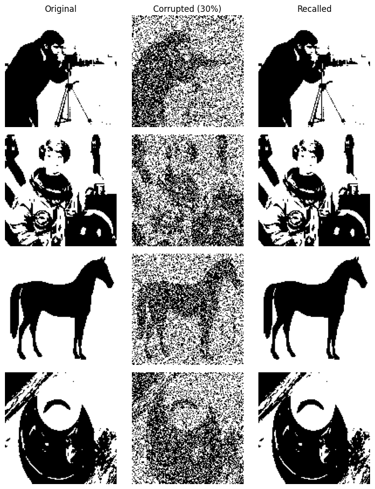
Step 6: Visualize Results

import matplotlib.pyplot as plt

def reshape_for_display(pattern, size=128):
    """Reshape 1D pattern back to 2D image."""
    return pattern.reshape(size, size)

# Plot original, corrupted, and recalled patterns
fig, axes = plt.subplots(len(training_data), 3, figsize=(8, 10))

for i in range(len(training_data)):
    # Column 1: Original training image
    axes[i, 0].imshow(reshape_for_display(training_data[i]), cmap='gray')
    axes[i, 0].axis('off')
    if i == 0:
        axes[i, 0].set_title('Original')

    # Column 2: Corrupted test input
    axes[i, 1].imshow(reshape_for_display(test_patterns[i]), cmap='gray')
    axes[i, 1].axis('off')
    if i == 0:
        axes[i, 1].set_title('Corrupted (30%)')

    # Column 3: Recalled output
    axes[i, 2].imshow(reshape_for_display(recalled[i]), cmap='gray')
    axes[i, 2].axis('off')
    if i == 0:
        axes[i, 2].set_title('Recalled')

plt.tight_layout()
plt.savefig('hopfield_memory_recall.png', dpi=150)
plt.show()

print("Visualization saved!")

Visualization saved!

Expected result:

• Original images are clean

• Corrupted inputs have ~30% noise

• Recalled outputs match originals (noise corrected!)

Complete Runnable Code

Here’s the full example in one block:

import numpy as np
import skimage.data
from skimage.color import rgb2gray
from skimage.transform import resize
from skimage.filters import threshold_mean
from matplotlib import pyplot as plt

from canns.models.brain_inspired import AmariHopfieldNetwork  # :cite:p:`amari1977neural,hopfield1982neural`
from canns.trainer import HebbianTrainer

np.random.seed(42)

# 1. Preprocess images
def preprocess_image(img, size=128):
    if img.ndim == 3:
        img = rgb2gray(img)
    img = resize(img, (size, size), anti_aliasing=True)
    thresh = threshold_mean(img)
    binary = img > thresh
    pattern = np.where(binary, 1.0, -1.0).astype(np.float32)
    return pattern.reshape(size * size)

camera = preprocess_image(skimage.data.camera())
astronaut = preprocess_image(skimage.data.astronaut())
horse = preprocess_image(skimage.data.horse().astype(np.float32))
coffee = preprocess_image(skimage.data.coffee())

training_data = [camera, astronaut, horse, coffee]

# 2. Create model and trainer (auto-initializes)
model = AmariHopfieldNetwork(num_neurons=training_data[0].shape[0], asyn=False, activation="sign")
trainer = HebbianTrainer(model)

# 3. Train
trainer.train(training_data)

# 4. Create corrupted test patterns
def corrupt_pattern(pattern, noise_level=0.3):
    corrupted = np.copy(pattern)
    num_flips = int(len(pattern) * noise_level)
    flip_indices = np.random.choice(len(pattern), num_flips, replace=False)
    corrupted[flip_indices] *= -1
    return corrupted

test_patterns = [corrupt_pattern(p, 0.3) for p in training_data]

# 5. Recall patterns
recalled = trainer.predict_batch(test_patterns, show_sample_progress=True)

# 6. Visualize
def reshape(pattern, size=128):
    return pattern.reshape(size, size)

fig, axes = plt.subplots(len(training_data), 3, figsize=(8, 10))
for i in range(len(training_data)):
    axes[i, 0].imshow(reshape(training_data[i]), cmap='gray')
    axes[i, 0].axis('off')
    axes[i, 1].imshow(reshape(test_patterns[i]), cmap='gray')
    axes[i, 1].axis('off')
    axes[i, 2].imshow(reshape(recalled[i]), cmap='gray')
    axes[i, 2].axis('off')

axes[0, 0].set_title('Original')
axes[0, 1].set_title('Corrupted')
axes[0, 2].set_title('Recalled')

plt.tight_layout()
plt.savefig('hopfield_memory.png')
plt.show()

CANN vs. Deep Learning Training

Aspect	Hebbian Learning	Deep Learning (ANNs)
Learning rule	Local (Hebbian, STDP [24])	Global (Backpropagation)
Supervision	Unsupervised	Supervised (usually)
Gradient	No gradient computation	Requires autodiff
Training data	Patterns to memorize	Labeled input-output pairs
Objective	Form attractors	Minimize loss function
Biological plausibility	High	Low
Speed	Fast (one-shot learning possible)	Slow (many epochs)
Capacity	Limited (~0.15N patterns for N neurons)	Very large (overparameterization)

When to use each:

• Hebbian/CANNs: Associative memory, pattern completion, neuroscience modeling

• Backprop/ANNs: Classification, regression, large-scale pattern recognition

The Trainer Abstraction

The Trainer framework provides a consistent interface across different learning paradigms:

# All trainers follow this pattern
trainer = SomeTrainer(model)
trainer.train(data)
output = trainer.predict(input)