Analysis Methods
This document explains the analysis and visualization tools in the CANNs library.
Overview
The analyzer module (canns.analyzer) provides tools for visualizing and interpreting both simulation outputs and experimental data. It organizes into distinct components based on data source and analysis type:
Module Structure
New Organization (v2.0+)
The analyzer module is organized by function:
metrics/ - Computational analysis (no matplotlib dependency)
spatial_metrics- Spatial metrics computationutils- Spike train conversion utilitiesexperimental/- CANN1D/2D experimental data analysis
visualization/ - Plotting and animation (matplotlib-based)
config- PlotConfig unified configuration systemspatial_plots- Spatial visualizationsenergy_plots- Energy landscape visualizationsspike_plots- Raster plots and firing rate plotstuning_plots- Tuning curve visualizationsexperimental/- Experimental data visualizations
slow_points/ - Fixed point analysis
model_specific/ - Specialized model analyzers
Analyze CANN simulation outputs
Analyze experimental neural recordings
Study fixed points and slow manifolds
Detect geometric structures in neural activity
Model Analyzer
The Model Analyzer visualizes the outputs of CANN simulations, focusing on network activity patterns and their evolution over time.
Core Capabilities
|
Animate firing rate evolution over time |
|
Snapshot of current activity pattern |
|
Track bump center position |
|
Visualize attractor basin structure |
|
Two-dimensional energy surface |
Purpose |
Show how different states relate to attractor minima |
|
Visualize recurrent connections |
|
Single neuron’s connectivity pattern |
Purpose |
Reveal Mexican-hat or other kernel structures |
Design Philosophy
Important
Model Analyzer functions receive simulation results as arrays rather than model objects. This independence means:
Same visualizations work across different model types
Results can be saved and analyzed later
No dependency on model internal structure during analysis
Functions accept standardized formats:
Firing rates as
(time, neurons)arraysMembrane potentials as
(time, neurons)arraysSpatial coordinates for bump localization
PlotConfig System
Configuration Pattern
The library uses PlotConfig dataclasses for visualization configuration:
Benefits:
✅ Reusability: Same configuration applies to multiple plots
✅ Type Safety: Parameters validated at construction
✅ Sharing: Pass configuration objects between functions
Common configuration includes:
figsize: Figure dimensionsinterval: Animation speedcolormap: Color scheme selectionshow_colorbar: Toggle color legend
While PlotConfig provides convenience, direct parameter passing remains supported for backward compatibility.
Data Analyzer
The Data Analyzer processes experimental neural recordings, typically spike trains or firing rate estimates.
Key Differences from Model Analyzer
Aspect |
Model Analyzer |
Data Analyzer |
|---|---|---|
Input Data |
Clean simulation outputs |
Spike trains—sparse, discrete events—and firing rate estimates |
Focus |
Visualize CANN dynamics |
Decode neural activity, fit parametric models |
Noise |
Minimal (simulation) |
Potentially noisy or incomplete recordings |
Capabilities
Estimate bump position from neural population
Fit Gaussian profiles to activity patterns
Track decoded position over time
Create synthetic spike trains for algorithm testing
Generate ground truth scenarios
Validate analysis pipelines
Tuning curve estimation
Circular statistics for angular variables
Error quantification metrics
Validate CANN models against experimental recordings
Develop decoding algorithms for neural data
Test theoretical predictions with simulated experiments
ASA Pipeline
The ASA (Attractor Structure Analyzer) pipeline is the main data-analysis workflow
for spike trains or firing-rate matrices with optional behavioral trajectories
(spike/x/y/t). It is available through the Python API and the ASA GUI.
Preprocessing |
|
Time TDA |
|
Decoding |
|
CohoMap |
|
CohoSpace |
|
PathCompare |
|
FR / FRM / GridScore |
Firing-rate heatmaps, single-neuron firing-rate maps, and gridness analysis. |
Time TDA and Spatial TDA
ASA now separates two point-cloud constructions:
Method |
Input point cloud |
Main use |
|---|---|---|
Time TDA |
Time samples of population activity, |
Dynamics, decoding, CohoMap/CohoSpace, and path comparison. |
Spatial TDA |
Position-binned firing-rate vectors, |
Spatial representation manifolds and Fig.4C-style barcode analysis. |
Spatial TDA is implemented by spatial_embedding.py and spatial_tda.py in
canns.analyzer.data.asa. The example script
examples/experimental_data_analysis/spatial_tda_from_asa.py provides a CLI wrapper
for ASA .npz files.
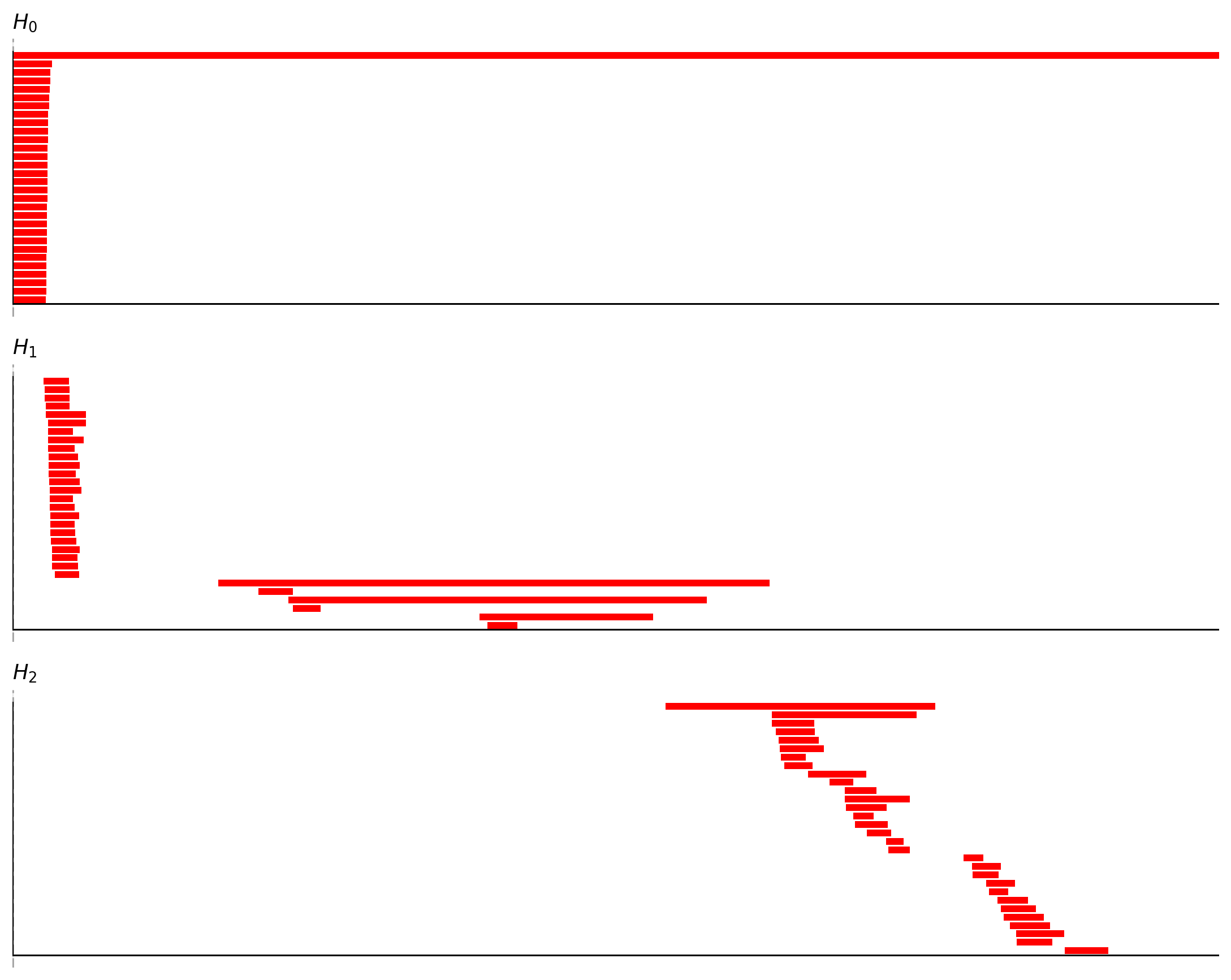
Example Spatial TDA output. This workflow first rewrites time-indexed activity
as position-indexed firing-rate vectors, r(x), then computes persistent
homology on the spatial-bin point cloud.
Workflow Helpers
Higher-level ASA workflows live in canns.analyzer.workflows. They compose existing
ASA building blocks rather than introducing separate low-level algorithms:
auto_grid_threshold.pysweeps grid-score ranked neuron subsets and reports candidate thresholds.phase_center_comparison.pycompares phase centers across sessions or conditions, using torus-aware displacement.
These helpers organize common research questions around the existing ASA modules:
Workflow |
Question |
Typical outputs |
|---|---|---|
|
Which grid-score cutoff or top-k subset gives a cleaner neuron population for TDA or coho analysis? |
Threshold sweep summaries, best subset metadata, barcode / coho quality metrics. |
|
How do the same neurons move in coho torus phase space across two sessions or conditions? |
Paired black/red phase-center plots and torus-aware displacement summaries. |
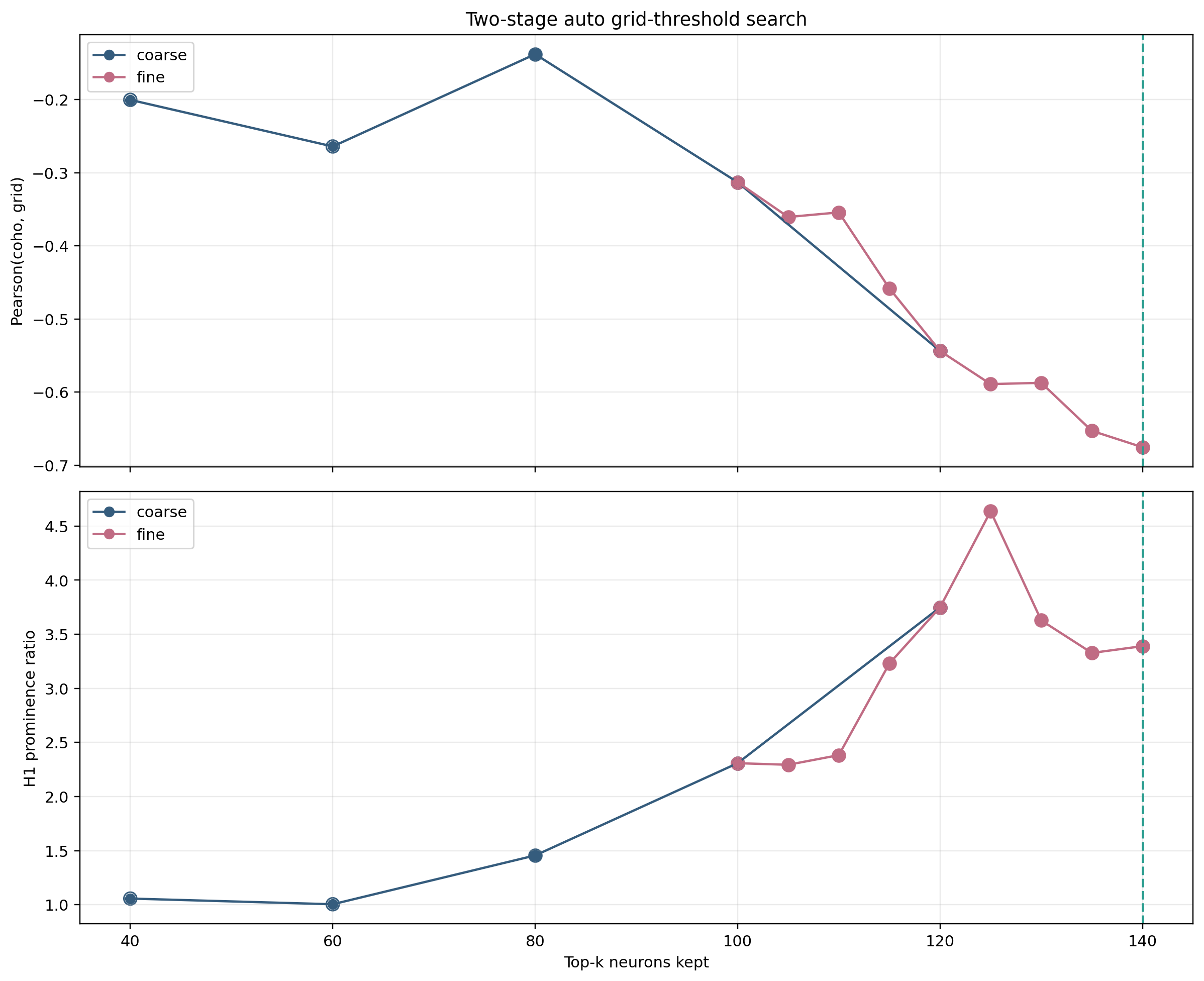
Example automatic grid-score threshold sweep. The workflow scans candidate subsets so users can quickly inspect which neuron population gives more stable topology and coho outputs.
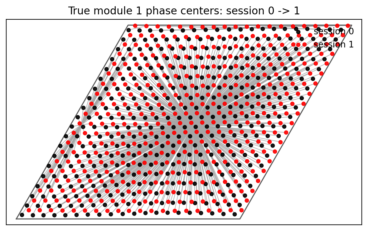
Example phase-center comparison. Black and red points mark the same neurons across two sessions or conditions, and connecting lines use the shortest displacement under torus periodic boundaries.
RNN Dynamics Analysis
This component analyzes recurrent neural networks as dynamical systems [31], finding fixed points [32] and characterizing the phase space structure.
Purpose
Note
CANN models are continuous-time dynamical systems. Understanding their behavior requires:
Identifying stable fixed points (attractors)
Finding unstable fixed points (saddles, repellers)
Mapping slow manifolds where dynamics concentrate
Methods
Locate states where dynamics vanish (du/dt = 0):
Numerical root finding
Multiple initial conditions for thorough search
Classification by stability (eigenvalue analysis)
Characterize dynamics near fixed points:
Jacobian computation
Eigenvalue decomposition
Attractor vs. saddle vs. repeller classification
Find low-dimensional structures in state space:
Dimensionality reduction
Identify directions of slow dynamics
Visualize state space organization
Current Scope
Implementation Status
Currently focused on analyzing RNN models (including CANNs as a special case). Provides tools for:
Understanding intrinsic network dynamics
Characterizing attractor landscapes
Studying bifurcations under parameter changes
Topological Data Analysis (TDA)
TDA tools [15] detect geometric and topological structures in high-dimensional neural activity data using persistent homology [16].
Why TDA for CANNs
Important
CANN activity patterns often live on low-dimensional manifolds:
Ring attractors: Activity on a circle (1D torus)
Torus attractors: Activity on a 2D torus (grid cells)
Sphere attractors: Activity on a sphere
Traditional methods may miss these structures. TDA provides mathematically rigorous detection.
Available Tools
Accelerated ripser implementation
Detects topological features (loops, voids)
Persistence diagrams quantify feature significance
User applies external tools (UMAP, PCA, etc.)
Library provides preprocessing utilities
Visualization of reduced representations
Use Cases
Grid cells encode position on a torus. TDA can:
For unknown networks:
✅ Infer attractor geometry from activity patterns
✅ Test hypotheses about encoding manifolds
✅ Compare experimental data with model predictions
Implementation Notes
Summary
The analysis module provides comprehensive tools for:
1️⃣
Model Analyzer: Visualize CANN simulation outputs with standardized functions
2️⃣
Data Analyzer: Process experimental recordings and synthetic neural data
3️⃣
RNN Dynamics: Study fixed points and phase space structure
4️⃣
TDA: Detect topological properties of neural representations
These tools enable both forward modeling (simulation analysis) and reverse engineering (experimental data interpretation)—supporting the full research cycle from theory to validation.