Tutorial 3: Analysis and Visualization Methods
This tutorial introduces visualization and analysis methods in the CANNs analyzer module.
1. Analyzer Module and PlotConfigs Overview
The canns.analyzer.plotting module provides visualization methods for analyzing simulation results. All plotting functions use the PlotConfigs system for unified configuration management.
1.1 Available Plotting Methods
1D Model Analysis:
energy_landscape_1d_static—Static energy landscapeenergy_landscape_1d_animation—Animated energy landscaperaster_plot—Spike raster plotaverage_firing_rate_plot—Average firing rate over timetuning_curve—Neural tuning curve
2D Model Analysis:
energy_landscape_2d_static—2D static energy landscapeenergy_landscape_2d_animation—2D animated energy landscape
1.2 PlotConfigs System
PlotConfigs provides method-specific configuration builders. Each plotting method has a corresponding config builder:
from canns.analyzer.visualization import (
PlotConfigs,
energy_landscape_1d_static,
energy_landscape_1d_animation,
raster_plot,
average_firing_rate_plot,
tuning_curve,
)
# Create configuration for each method
config_static = PlotConfigs.energy_landscape_1d_static(
figsize=(10, 6),
title='Energy Landscape',
show=True, # Display plot (default)
save_path=None # Don't save to file (default)
)
# Use configuration with plotting function
energy_landscape_1d_static(
data_sets={'r': (model.x, r_history)},
config=config_static
)
Note
This is a conceptual example. The actual usage will be demonstrated in Section 2 below with real data.
Key Benefits:
Unified Interface: All plotting methods follow the same pattern
Configuration Reuse: Create once, use multiple times
Clear Defaults:
show=True, save_path=Nonefor interactive visualization
Note
By default, plots are displayed (show=True) and not saved (save_path=None). Set save_path='filename.png' to save plots.
2. 1D Analysis Methods
Let’s demonstrate all 1D analysis methods using a SmoothTracking1D task.
2.1 Preparation
[1]:
import brainpy.math as bm
from canns.models.basic import CANN1D
from canns.task.tracking import SmoothTracking1D
from canns.analyzer.visualization import (
PlotConfigs,
energy_landscape_1d_static,
energy_landscape_1d_animation,
raster_plot,
average_firing_rate_plot,
tuning_curve,
)
# Setup environment
bm.set_dt(0.1)
# Create model
model = CANN1D(num=256, tau=1.0, k=8.1, a=0.5, A=10, J0=4.0)
# Create smooth tracking task
# Stimulus moves from -2.0 to 2.0, then to -1.0
task = SmoothTracking1D(
cann_instance=model,
Iext=[-4.0, 4.0, -2.0, 2.0], # Keypoint positions
duration=[20.0, 30.0, 20.0], # Duration for each segment
time_step=bm.get_dt(),
)
# Get task data
task.get_data()
# Define simulation step
def run_step(t, inp):
model.update(inp)
return model.u.value, model.r.value, model.inp.value
# Run simulation
u_history, r_history, input_history = bm.for_loop(run_step, operands=(task.run_steps, task.data), progress_bar=10)
<SmoothTracking1D> Generating Task data: 700it [00:00, 1633.05it/s]
2.2 Energy Landscape (Static)
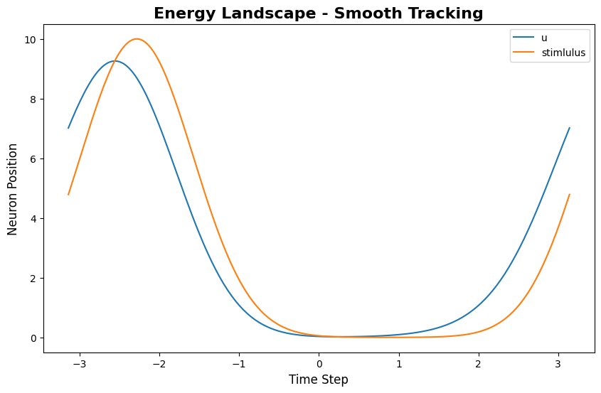
energy_landscape_1d_static plots firing rate over time and neuron position:
[2]:
index = 200 # Time step to visualize
# Configure static energy landscape
config_static = PlotConfigs.energy_landscape_1d_static(
figsize=(10, 6),
title='Energy Landscape - Smooth Tracking',
xlabel='Time Step',
ylabel='Neuron Position',
show=True,
save_path=None
)
# Plot static energy landscape
energy_landscape_1d_static(
data_sets={'u': (model.x, u_history[index]), 'stimlulus': (model.x, input_history[index])},
config=config_static
)
[2]:
(<Figure size 1000x600 with 1 Axes>,
<Axes: title={'center': 'Energy Landscape - Smooth Tracking'}, xlabel='Time Step', ylabel='Neuron Position'>)
This shows the bump trajectory over time: x-axis is time, y-axis is feature space position, color intensity represents firing rate.
2.3 Energy Landscape (Animation)
energy_landscape_1d_animation generates a dynamic animation showing bump evolution:
[3]:
# Configure animation
config_anim = PlotConfigs.energy_landscape_1d_animation(
time_steps_per_second=100, # 100 time steps = 1 second of real time
fps=20, # 20 frames per second
title='Energy Landscape Animation',
xlabel='Neuron Position',
ylabel='Firing Rate',
repeat=True,
show=True,
save_path=None # Set to 'animation.gif' to save
)
# Generate animation
energy_landscape_1d_animation(
data_sets={'u': (model.x, u_history), 'stimlulus': (model.x, input_history)},
config=config_anim
)
Animation Parameters:
- time_steps_per_second: How many simulation time steps per real-world second
- fps: Frames per second for the animation
- repeat: Whether to loop the animation
2.4 Raster Plot
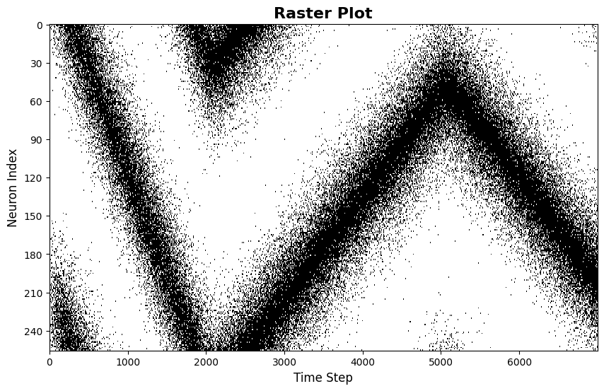
raster_plot shows spike timing of neurons:
[4]:
from canns.analyzer.metrics.utils import firing_rate_to_spike_train
# Configure raster plot
config_raster = PlotConfigs.raster_plot(
figsize=(10, 6),
title='Raster Plot',
xlabel='Time Step',
ylabel='Neuron Index',
show=True,
save_path=None
)
# use u to generate spike train, because it has higher values
spike_train = firing_rate_to_spike_train(u_history, dt_spike=0.01, dt_rate=bm.get_dt())
# Plot raster
raster_plot(
spike_train=spike_train,
config=config_raster
)
[4]:
(<Figure size 1000x600 with 1 Axes>,
<Axes: title={'center': 'Raster Plot'}, xlabel='Time Step', ylabel='Neuron Index'>)
Each dot represents a neuron firing at a specific time. The pattern reveals the bump’s spatial structure and temporal evolution.
2.5 Average Firing Rate Plot
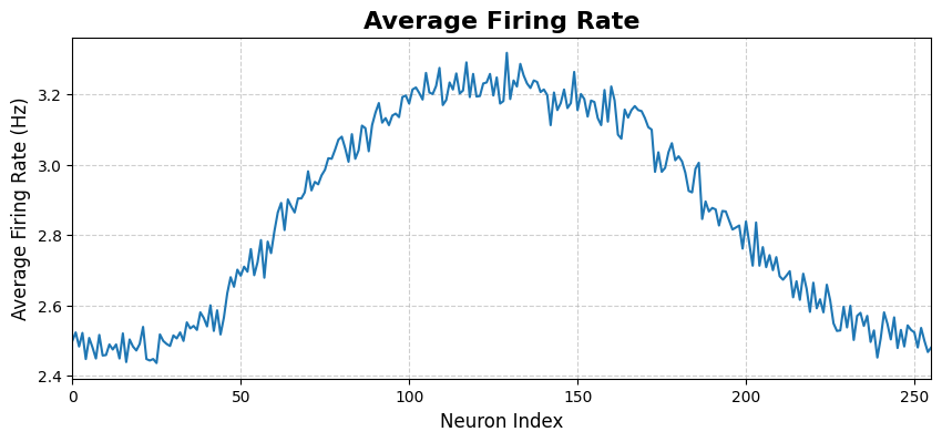
average_firing_rate_plot shows population-averaged firing rate over time:
[5]:
# Configure average firing rate plot
config_avg = PlotConfigs.average_firing_rate_plot(
figsize=(10, 4),
title='Average Firing Rate',
xlabel='Time (ms)',
ylabel='Average Firing Rate',
show=True,
save_path=None
)
# Plot average firing rate
average_firing_rate_plot(
spike_train=spike_train,
dt=bm.get_dt(),
config=config_avg
)
[5]:
(<Figure size 1000x400 with 1 Axes>,
<Axes: title={'center': 'Average Firing Rate'}, xlabel='Neuron Index', ylabel='Average Firing Rate (Hz)'>)
This plot shows the overall activity level of the network over time.
2.6 Tuning Curve
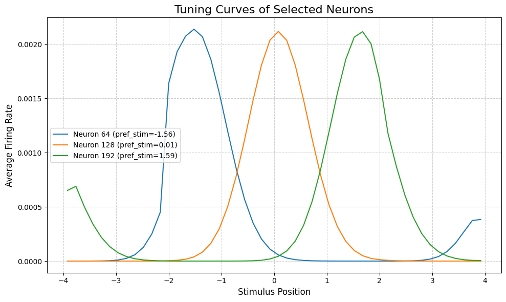
tuning_curve shows individual neurons’ responses to different stimulus positions:
[6]:
# Configure tuning curve
config_tuning = PlotConfigs.tuning_curve(
num_bins=50, # Number of position bins
pref_stim=model.x, # Preferred stimuli for each neuron
title='Tuning Curves of Selected Neurons',
xlabel='Stimulus Position',
ylabel='Average Firing Rate',
show=True,
save_path=None,
)
# Select neurons to plot
neuron_indices = [64, 128, 192] # Left, center, right
# Plot tuning curves
tuning_curve(
stimulus=task.Iext_sequence.squeeze(),
firing_rates=r_history,
neuron_indices=neuron_indices,
config=config_tuning
)
[6]:
(<Figure size 1000x600 with 1 Axes>,
<Axes: title={'center': 'Tuning Curves of Selected Neurons'}, xlabel='Stimulus Position', ylabel='Average Firing Rate'>)
The tuning curve reveals each neuron’s “preferred position”—the stimulus location that elicits maximum response. For CANN models, neurons typically have bell-shaped tuning curves centered at different positions.
3. Energy Landscapes for Different Tasks
Different tasks produce characteristic energy landscape patterns. Let’s compare three tracking tasks:
3.1 PopulationCoding1D
Population coding demonstrates memory maintenance after brief stimulus presentation.
[7]:
from canns.task.tracking import PopulationCoding1D
model = CANN1D(num=256, tau=1.0, k=8.1, a=0.5, A=10, J0=4.0)
# Population coding task
task_pc = PopulationCoding1D(
cann_instance=model,
before_duration=10.0,
after_duration=10.0,
Iext=0.0,
duration=20.0,
time_step=bm.get_dt(),
)
# Get data and run simulation
task_pc.get_data()
u_pc, r_pc, inp_pc = bm.for_loop(run_step, operands=(task_pc.run_steps, task_pc.data), progress_bar=10)
# Visualize
config_anim = PlotConfigs.energy_landscape_1d_animation(
time_steps_per_second=100, # 100 time steps = 1 second of real time
fps=20, # 20 frames per second
title='Energy Landscape Animation - Population Coding',
xlabel='Neuron Position',
ylabel='Firing Rate',
repeat=True,
show=True,
save_path=None # Set to 'animation.gif' to save
)
# Generate animation
energy_landscape_1d_animation(
data_sets={'u': (model.x, u_pc), 'stimlulus': (model.x, inp_pc)},
config=config_anim
)
<PopulationCoding1D>Generating Task data(No For Loop)
Characteristic Pattern: The bump forms during stimulus presentation (middle section) and persists at the same location after stimulus ends (right section). This demonstrates the attractor’s stability and memory maintenance capability.
3.2 TemplateMatching1D
Template matching demonstrates pattern completion from noisy input.
[8]:
from canns.task.tracking import TemplateMatching1D
model = CANN1D(num=256, tau=1.0, k=8.1, a=0.5, A=10, J0=4.0)
# Template matching task
task_tm = TemplateMatching1D(
cann_instance=model,
Iext=1.0,
duration=50.0,
time_step=bm.get_dt(),
)
# Get data and run simulation
task_tm.get_data()
u_tm, r_tm, inp_tm = bm.for_loop(run_step, operands=(task_tm.run_steps, task_tm.data), progress_bar=10)
# Visualize
config_anim = PlotConfigs.energy_landscape_1d_animation(
time_steps_per_second=100, # 100 time steps = 1 second of real time
fps=20, # 20 frames per second
title='Energy Landscape Animation - Template Matching',
xlabel='Neuron Position',
ylabel='Firing Rate',
repeat=True,
show=True,
save_path=None # Set to 'animation.gif' to save
)
# Generate animation
energy_landscape_1d_animation(
data_sets={'u': (model.x, u_tm), 'stimlulus': (model.x, inp_tm)},
config=config_anim
)
<TemplateMatching1D>Generating Task data: 100%|██████████| 500/500 [00:00<00:00, 10877.85it/s]
Characteristic Pattern: Initially distributed activity (noisy input creates broad, weak activation) converges to a single sharp bump. This demonstrates the attractor’s ability to “clean up” noisy inputs through convergence.
3.3 SmoothTracking1D
Smooth tracking demonstrates the bump following a moving stimulus.
[9]:
from canns.task.tracking import SmoothTracking1D
model = CANN1D(num=256, tau=1.0, k=8.1, a=0.5, A=10, J0=4.0)
# Smooth tracking task
task_st = SmoothTracking1D(
cann_instance=model,
Iext=[-2.0, 2.0],
duration=[50.0],
time_step=bm.get_dt(),
)
# Get data and run simulation
task_st.get_data()
u_st, r_st, inp_st = bm.for_loop(run_step, operands=(task_st.run_steps, task_st.data), progress_bar=10)
# Visualize
config_anim = PlotConfigs.energy_landscape_1d_animation(
time_steps_per_second=100, # 100 time steps = 1 second of real time
fps=20, # 20 frames per second
title='Energy Landscape Animation - Smooth Tracking',
xlabel='Neuron Position',
ylabel='Firing Rate',
repeat=True,
show=True,
save_path=None # Set to 'animation.gif' to save
)
# Generate animation
energy_landscape_1d_animation(
data_sets={'u': (model.x, u_st), 'stimlulus': (model.x, inp_st)},
config=config_anim
)
<SmoothTracking1D> Generating Task data: 500it [00:00, 6982.24it/s]
Characteristic Pattern: The bump smoothly moves from left to right, tracking the moving stimulus. This demonstrates the attractor’s ability to integrate external input while maintaining stable bump structure.
3.4 Comparison Summary
Task |
Input Pattern |
Energy Landscape Feature |
Demonstrates |
|---|---|---|---|
PopulationCoding |
Brief stimulus |
Bump forms and persists in place |
Memory maintenance |
TemplateMatching |
Noisy continuous input |
Distributed activity → Sharp bump |
Pattern completion |
SmoothTracking |
Moving stimulus |
Bump smoothly follows trajectory |
Stimulus tracking |
These three patterns illustrate the three key computational capabilities of continuous attractor networks: memory, denoising, and tracking.
4. 2D Analysis Methods
For CANN2D models, the analyzer provides corresponding 2D visualization methods. The PlotConfigs pattern works identically for 2D visualizations.
4.1 Preparing CANN2D Simulation
[ ]:
from canns.models.basic import CANN2D
from canns.task.tracking import SmoothTracking2D
from canns.analyzer.visualization import (
PlotConfigs,
energy_landscape_2d_static,
energy_landscape_2d_animation,
)
# Create 2D model
model_2d = CANN2D(
length=32, # 32x32 neuron grid
tau=1.0,
k=8.1,
a=0.3,
A=10,
J0=4.0,
)
# Create 2D tracking task
# Move from (-1, -1) to (1, 1) to (-1, 1)
task_2d = SmoothTracking2D(
cann_instance=model_2d,
Iext=[(-1.0, -1.0), (1.0, 1.0), (-1.0, 1.0)],
duration=[30.0, 30.0],
time_step=0.1,
)
# Get data and run simulation
task_2d.get_data()
def run_step_2d(t, inp):
model_2d.update(inp)
return model_2d.u.value, model_2d.r.value
u_history_2d, r_history_2d = bm.for_loop(run_step_2d, operands=(task_2d.run_steps, task_2d.data), progress_bar=10)
<SmoothTracking2D> Generating Task data: 600it [00:00, 1153.29it/s]
4.2 Energy Landscape 2D (Static)
[11]:
# Select a time point to visualize
time_idx = 300
# Configure 2D static landscape
config_2d_static = PlotConfigs.energy_landscape_2d_static(
figsize=(8, 8),
title=f'2D Energy Landscape at t={time_idx * 0.1:.1f}',
xlabel='X Position',
ylabel='Y Position',
show=True,
save_path=None
)
# Plot 2D energy landscape at specific time
energy_landscape_2d_static(
z_data=u_history_2d[time_idx],
config=config_2d_static
)
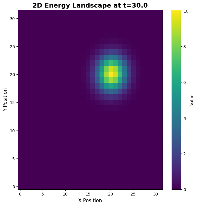
[11]:
(<Figure size 800x800 with 2 Axes>,
<Axes: title={'center': '2D Energy Landscape at t=30.0'}, xlabel='X Position', ylabel='Y Position'>)
The 2D static plot shows the spatial distribution of firing rates at a single time point, revealing the 2D bump structure.
4.3 Energy Landscape 2D (Animation)
[12]:
# Configure 2D animation
config_2d_anim = PlotConfigs.energy_landscape_2d_animation(
time_steps_per_second=100,
fps=20,
figsize=(8, 8),
title='2D Energy Landscape Animation',
xlabel='X Position',
ylabel='Y Position',
repeat=True,
show=True,
save_path=None # Set to 'animation_2d.gif' to save
)
# Generate 2D energy landscape animation
energy_landscape_2d_animation(
zs_data=u_history_2d,
config=config_2d_anim
)
The 2D animation shows the bump moving through the 2D feature space, following the trajectory defined by the task.
5. Next Steps
Congratulations on completing Tutorial 3! You now know: - How to use PlotConfigs for unified visualization configuration - All major 1D and 2D visualization methods in CANNs - How different tasks produce characteristic energy landscape patterns - The three key computational capabilities: memory, denoising, and tracking
Continue Learning
Next: Tutorial 4: Parameter Effects—Explore how parameters systematically affect model behavior
For Advanced Applications: Continue with Tutorials 5-7 for hierarchical models and brain-inspired networks
Key Takeaways
PlotConfigs Pattern: Always use
PlotConfigs.method_name()to create configuration, then pass to plotting functionsDefault Behavior: Plots display by default (
show=True, save_path=None)Data Sets: All plotting functions accept
data_setsdictionary for flexible data inputTask Patterns: Different tasks reveal different attractor properties (stability, convergence, tracking)