教程 6:层级化路径积分网络
本教程介绍层级化路径积分网络,该网络结合多尺度网格细胞 [2],以实现大环境中的鲁棒空间导航。
Important
参考文献
本教程实现的模型来自:Chu et al. (2025)——“Localized Space Coding and Phase Coding Complement Each Other to Achieve Robust and Efficient Spatial Representation” [19]
如需详细的理论背景与实验验证,请参阅原始论文。
1. 分层路径积分简介
1.1 什么是分层路径积分?
路径积分是指通过随时间积分自我运动信号(速度)来追踪位置的能力。层级化路径积分 [4, 28] [19] 利用多个在不同空间尺度上运行的网格细胞 [2] 模块,实现以下目标:
多尺度表征:粗尺度用于大范围空间,细尺度用于高精度定位
误差校正:多尺度结构提供冗余,以对抗漂移误差
高效编码:不同模块以不同分辨率对空间进行平铺
1.2 生物学启发
在哺乳动物大脑中:
1.3 关键组件
该分层网络由以下部分组成:
2. 模型架构
2.1 组件概览
[ ]:
from canns.models.basic import HierarchicalNetwork

# Create hierarchical network with 5 modules
hierarchical_net = HierarchicalNetwork(
    num_module=5,        # Number of grid modules (different scales)
    num_place=30,        # Place cells per dimension (30x30 = 900 total)
    spacing_min=2.0,     # Smallest grid spacing
    spacing_max=5.0,     # Largest grid spacing
    module_angle=0.0     # Base orientation angle
)
2.2 关键参数
参数 |
类型 |
描述 |
|---|---|---|
|
int |
具有不同尺度的网格模块数量 |
|
int |
每个空间维度上的位置细胞数量 |
|
float |
最小网格间距(最精细尺度) |
|
float |
最大网格间距(最粗糙尺度) |
|
float |
网格模块的基础朝向角 |
参数建议:
num_module=5:在覆盖范围与计算开销之间取得良好平衡num_place=30:为 5×5 米环境提供 900 个位置细胞间距范围应与环境尺寸匹配(更大空间需更大的
spacing_max)
2.3 内部结构
每个模块包含:
3 个带状细胞网络,分别对应 0°、60°、120° 三个方向
1 个网格细胞网络,整合来自带状细胞的输出
连接投影至共享的位置细胞群体
3. 完整示例:多尺度导航
3.1 设置与任务创建
[14]:
import brainpy.math as bm
import numpy as np
from canns.models.basic import HierarchicalNetwork
from canns.task.open_loop_navigation import OpenLoopNavigationTask
# Setup environment
bm.set_dt(0.05)
# Create navigation task (5m x 5m environment)
task = OpenLoopNavigationTask(
width=5.0, # Environment width (meters)
height=5.0, # Environment height (meters)
speed_mean=0.04, # Mean speed (m/step)
speed_std=0.016, # Speed standard deviation
duration=50000.0, # Simulation duration (steps)
dt=0.05, # Time step
start_pos=(2.5, 2.5), # Start at center
progress_bar=True
)
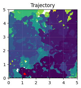
# Generate trajectory data
task.get_data()
print(f"Trajectory: {task.data.position.shape[0]} steps")
print(f"Environment: {task.width}m x {task.height}m")
task.show_data()
<OpenLoopNavigationTask>Generating Task data: 100%|██████████| 1000000/1000000 [00:00<00:00, 1468708.52it/s]
Trajectory: 1000000 steps
Environment: 5.0m x 5.0m
3.2 创建层级化网络
[3]:
# Create hierarchical network
hierarchical_net = HierarchicalNetwork(
    num_module=5,         # 5 different spatial scales
    num_place=30,         # 30x30 place cell grid
    spacing_min=2.0,      # Finest grid scale
    spacing_max=5.0,      # Coarsest grid scale
)
3.3 初始化阶段
关键步骤:使用强位置输入初始化网络,以设定初始位置。
[4]:
def initialize(t, input_strength):
    """Initialize network with location input"""
    hierarchical_net(
        velocity=bm.zeros(2,),        # No velocity during init
        loc=task.data.position[0],        # Starting position
        loc_input_stre=input_strength,    # Input strength
    )

# Create initialization schedule
init_time = 500
indices = np.arange(init_time)
input_strength = np.zeros(init_time)
input_strength[:400] = 100.0  # Strong input for first 400 steps

# Run initialization
bm.for_loop(
    initialize,
    operands=(bm.asarray(indices), bm.asarray(input_strength)),
    progress_bar=10,
)

print("Initialization complete")
Running for 500 iterations: 100%|██████████| 500/500 [00:00<00:00, 1896.23it/s]
Initialization complete
为何初始化至关重要:
使所有网格模块处于一致的起始状态
强位置输入(100.0)锚定网络状态
若未正确初始化,各模块可能初始不同步
3.4 主模拟循环
[5]:
def run_step(t, vel, loc):
    """Single simulation step with velocity input"""
    hierarchical_net(
        velocity=vel,           # Current velocity
        loc=loc,                # Current position (for reference)
        loc_input_stre=0.0      # No location input during navigation
    )

    # Extract firing rates from all layers
    band_x_r = hierarchical_net.band_x_fr.value   # X-direction band cells
    band_y_r = hierarchical_net.band_y_fr.value   # Y-direction band cells
    grid_r = hierarchical_net.grid_fr.value       # Grid cells
    place_r = hierarchical_net.place_fr.value     # Place cells

    return band_x_r, band_y_r, grid_r, place_r

# Get trajectory data
total_time = task.data.velocity.shape[0]
indices = np.arange(total_time)

# Run simulation
print("Running main simulation...")
band_x_r, band_y_r, grid_r, place_r = bm.for_loop(
    run_step,
    operands=(
        bm.asarray(indices),
        bm.asarray(task.data.velocity),
        bm.asarray(task.data.position)
    ),
    progress_bar=10000,
)

print(f"Simulation complete!")
print(f"Band X cells: {band_x_r.shape}")
print(f"Band Y cells: {band_y_r.shape}")
print(f"Grid cells: {grid_r.shape}")
print(f"Place cells: {place_r.shape}")
Running main simulation...
Running for 1,000,000 iterations: 100%|██████████| 1000000/1000000 [07:18<00:00, 2278.48it/s]
Simulation complete!
Band X cells: (1000000, 5, 180)
Band Y cells: (1000000, 5, 180)
Grid cells: (1000000, 5, 400)
Place cells: (1000000, 900)
输出解释:
band_x_r:形状 (T, num_module, num_cells) —— X 方向的带状细胞活动band_y_r:形状 (T, num_module, num_cells) —— Y 方向的带状细胞活动grid_r:形状 (T, num_module, num_gc_x, num_gc_y) —— 网格细胞活动place_r:形状 (T, num_place, num_place) —— 位置细胞响应
4. 可视化与分析
4.1 计算发放场
发放场显示每个神经元在环境中活跃的位置:
[7]:
from canns.analyzer.metrics.spatial_metrics import compute_firing_field, gaussian_smooth_heatmaps
from canns.analyzer.visualization import PlotConfig, plot_firing_field_heatmap

# Prepare data
loc = np.array(task.data.position)
width = 5
height = 5
M = int(width * 10)
K = int(height * 10)

T = grid_r.shape[0]

# Reshape arrays for firing field computation
grid_r = grid_r.reshape(T, -1)
band_x_r = band_x_r.reshape(T, -1)
band_y_r = band_y_r.reshape(T, -1)
place_r = place_r.reshape(T, -1)

# Compute firing fields
print("Computing firing fields...")
heatmaps_grid = compute_firing_field(np.array(grid_r), loc, width, height, M, K)
heatmaps_band_x = compute_firing_field(np.array(band_x_r), loc, width, height, M, K)
heatmaps_band_y = compute_firing_field(np.array(band_y_r), loc, width, height, M, K)
heatmaps_place = compute_firing_field(np.array(place_r), loc, width, height, M, K)

# Apply Gaussian smoothing
heatmaps_grid = gaussian_smooth_heatmaps(heatmaps_grid)
heatmaps_band_x = gaussian_smooth_heatmaps(heatmaps_band_x)
heatmaps_band_y = gaussian_smooth_heatmaps(heatmaps_band_y)
heatmaps_place = gaussian_smooth_heatmaps(heatmaps_place)

print(f"Firing fields computed: {heatmaps_grid.shape}")
Computing firing fields...
Firing fields computed: (2000, 50, 50)
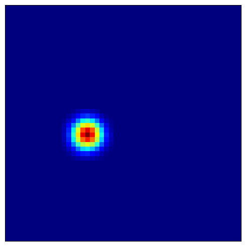
4.2 可视化网格细胞模式
网格细胞表现出特征性的六边形发放模式:
[9]:
# Reshape to separate modules
heatmaps_grid = heatmaps_grid.reshape(5, -1, M, K)  # (modules, cells, x, y)

# Visualize a grid cell from module 0
module_idx = 0
cell_idx = 42

config = PlotConfig(
    figsize=(6, 6),
    title=f'Grid Cell - Module {module_idx}, Cell {cell_idx}',
    xlabel='X Position (m)',
    ylabel='Y Position (m)',
    show=True,
    save_path=None
)

plot_firing_field_heatmap(
    heatmaps_grid[module_idx, cell_idx],
    config=config
)
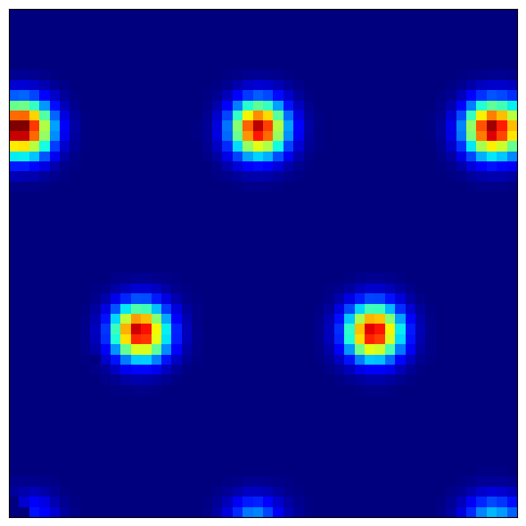
[9]:
(<Figure size 600x600 with 1 Axes>, <Axes: >)
观察要点:
模块 0 (最精细尺度):小型、密集排列的六边形
模块 4 (最粗糙尺度):大型、间距稀疏的六边形
规则间距:网格顶点构成等边三角形
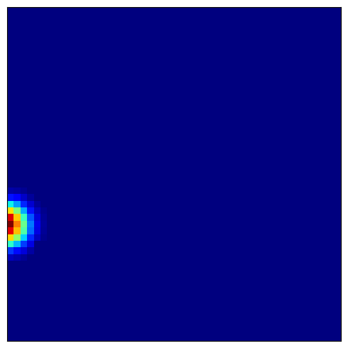
4.3 可视化带状细胞模式
[10]:
# Reshape band cells
heatmaps_band_x = heatmaps_band_x.reshape(5, -1, M, K)

# Visualize a band cell
config = PlotConfig(
    figsize=(6, 6),
    title=f'Band Cell X - Module {module_idx}, Cell {cell_idx}',
    xlabel='X Position (m)',
    ylabel='Y Position (m)',
    show=True,
    save_path=None
)

plot_firing_field_heatmap(
    heatmaps_band_x[module_idx, cell_idx],
    config=config
)
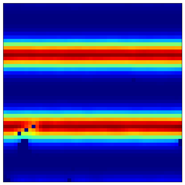
[10]:
(<Figure size 600x600 with 1 Axes>, <Axes: >)
预期模式:
平行条纹 垂直于偏好方向
不同细胞具有不同的条纹间距(相位偏移)
多个模块呈现不同尺度的条纹结构
4.4 可视化位置细胞场
位置细胞整合来自网格细胞的输入,形成局部化放电场:
[11]:
# Visualize several place cells
for place_idx in [100, 200, 300, 400]:
    config = PlotConfig(
        figsize=(5, 5),
        title=f'Place Cell {place_idx}',
        xlabel='X Position (m)',
        ylabel='Y Position (m)',
        show=True,
        save_path=None
    )

    plot_firing_field_heatmap(
        heatmaps_place[place_idx],
        config=config
    )
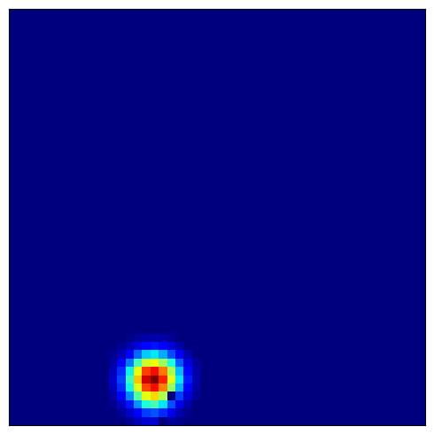
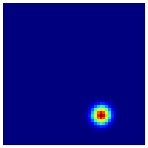
预期模式:
局部化场域:每个位置细胞仅在特定位置(或多个位置)放电
多放电场:部分细胞可能具有多个放电位置
环境覆盖:不同细胞共同覆盖整个空间环境
5. 后续步骤
恭喜!您已完成分层路径积分网络教程,现已理解:
多尺度网格细胞模块如何提供鲁棒的空间编码
带状细胞、网格细胞与位置细胞的组合架构
如何正确初始化分层网络
如何可视化不同空间尺度下的放电场
您所掌握的内容
继续学习
探索相关高级主题:
教程 6:Theta 扫描 HD-网格系统 —— 学习结合头朝向与网格细胞的 theta 调制系统
教程 7:Theta 扫描位置细胞网络 —— 理解在具有测地距离的复杂环境中位置细胞的编码机制
或探索其他场景:
场景 2:数据分析 —— 比较模型预测与实验数据
场景 3:类脑学习 —— 训练空间记忆系统
场景 4:流水线 —— 用于完整工作流的高级工具
核心要点
多尺度表征 —— 不同网格间距提供互补的位置信息
初始化至关重要 —— 必须使用强位置输入同步所有模块
带状细胞是基础单元 —— 网格细胞由不同朝向的带状细胞模块组合涌现
位置细胞整合信息 —— 通过组合网格细胞输入形成局部化放电场
高级主题
- 误差校正
多尺度结构允许网络校正累积漂移误差:细尺度检测微小偏差,粗尺度提供全局参考。
- 尺度特性
网格间距通常遵循几何级数(例如,5 个模块的间距为:2.0、2.5、3.1、3.9、4.9 米)。
- 生物参数
实际网格细胞间距范围约为 30 厘米至数米。请调整
spacing_min和spacing_max以匹配实验数据。- 位置场形成
在大环境中,由于网格细胞的周期性,位置细胞可能发展出多个放电场。
参数调优指南
对于分层网络:
num_module=5-7:在覆盖范围与计算开销间取得良好平衡spacing_min:匹配最精细实验网格间距(约 30–50 厘米)spacing_max:应覆盖环境尺寸(例如,5×5 米环境设为 5 米)num_place:提高分辨率以实现精细位置编码(每维度 30–50)
研究应用
该模型适用于:
路径积分研究 —— 动物如何通过自我运动追踪位置
网格细胞研究 —— 理解多尺度空间编码机制
海马体模型 —— 连接内嗅皮层输入与位置细胞形成
导航算法 —— 类生物机器人与自主系统设计
下一步:教程 6:Theta 扫描 HD-网格系统