RNN Fixed Point Analysis Tutorial: FlipFlop Task Example

Objective: This document serves as a comprehensive tutorial that explains how to use the FixedPointFinder tool to analyze an RNN trained on the FlipFlop task.

Structure: 1. Theoretical Background—What are fixed points? 2. Environment Setup—Import required libraries for the script 3. Component Definitions—Introduce FlipFlopData, FlipFlopRNN and train_flipflop_rnn functions one by one. 4. Core Usage—Demonstrate the concrete workflow of using FixedPointFinder.

1. Theoretical Background: What are Fixed Points?

Fixed Points [29, 30] are a core concept in dynamical systems. For an RNN, we can view it as a function h_t+1 = F(h_t, u_t), where h is the hidden state and u is the input.

When input ``u`` remains constant (e.g., during the “memory” phase in the FlipFlop task with no pulse input, u=0), the system evolves as h_t+1 = F(h_t).

A fixed point ``x*`` is a state that satisfies x* = F(x*). * Stable Fixed Point: Acts like an “attractor”. If the RNN state h gets close to x*, it will eventually settle at x*. * Unstable Fixed Point: Acts like a “repeller” or “saddle point”.

Core Principle: We train an RNN to complete the FlipFlop task. After successful training, the RNN learns to create a stable fixed point for each state it needs to “remember” (e.g., [+1, +1] or [+1, -1]). When the input u=0, the RNN state will automatically flow toward and settle at these fixed points, thereby achieving the “memory” function.

The purpose of this tutorial is to use the FixedPointFinder tool to discover all the stable fixed points that the RNN has “hidden” inside.

2. Imports

Import all libraries used in the flipflop_fixed_points.py script.

import brainpy as bp  # :cite:p:`wang2023brainpy`
import brainpy.math as bm
import jax  # :cite:p:`jax2018github`
import jax.numpy as jnp
import numpy as np
import random
from canns.analyzer.visualization import PlotConfig
from canns.analyzer.slow_points import FixedPointFinder, save_checkpoint, load_checkpoint, plot_fixed_points_2d, plot_fixed_points_3d

3. Component Definitions: Data, Model and Training

In this section, we define the three core components from the flipflop_fixed_points.py script.

3.1 Component 1: FlipFlopData Class

This is the FlipFlopData class from the flipflop_fixed_points.py script.

class FlipFlopData:
    """Generator for flip-flop memory task data."""

    def __init__(self, n_bits=3, n_time=64, p=0.5, random_seed=0):
        """Initialize FlipFlopData generator.

        Args:
            n_bits: Number of memory channels.
            n_time: Number of timesteps per trial.
            p: Probability of input pulse at each timestep.
            random_seed: Random seed for reproducibility.
        """
        self.rng = np.random.RandomState(random_seed)
        self.n_time = n_time
        self.n_bits = n_bits
        self.p = p

    def generate_data(self, n_trials):
        """Generate flip-flop task data.

        Args:
            n_trials: Number of trials to generate.

        Returns:
            dict with 'inputs' and 'targets' arrays [n_trials x n_time x n_bits].
        """
        n_time = self.n_time
        n_bits = self.n_bits
        p = self.p

        # Generate unsigned input pulses
        unsigned_inputs = self.rng.binomial(1, p, [n_trials, n_time, n_bits])

        # Ensure every trial starts with a pulse
        unsigned_inputs[:, 0, :] = 1

        # Generate random signs {-1, +1}
        random_signs = 2 * self.rng.binomial(1, 0.5, [n_trials, n_time, n_bits]) - 1

        # Apply random signs
        inputs = unsigned_inputs * random_signs

        # Compute targets
        targets = np.zeros([n_trials, n_time, n_bits])
        for trial_idx in range(n_trials):
            for bit_idx in range(n_bits):
                input_seq = inputs[trial_idx, :, bit_idx]
                t_flip = np.where(input_seq != 0)[0]
                for flip_idx in range(len(t_flip)):
                    t_flip_i = t_flip[flip_idx]
                    targets[trial_idx, t_flip_i:, bit_idx] = inputs[
                        trial_idx, t_flip_i, bit_idx
                    ]

        return {
            "inputs": inputs.astype(np.float32),
            "targets": targets.astype(np.float32),
        }

3.2 Component 2: FlipFlopRNN Class

This is the FlipFlopRNN class from the flipflop_fixed_points.py script.

Usage Notes: The principle of FixedPointFinder is to find x = F(x, u). To compute F(x, u), it will call rnn_model(inputs, hidden). FixedPointFinder will pass inputs with shape [batch, 1, n_inputs] and hidden with shape [batch, n_hidden].

Therefore, your __call__ method must be able to handle the case when n_time == 1 and return (outputs, h_next).

Please see the if n_time == 1: branch in the code below, which is specifically designed to adapt to FixedPointFinder.

Note: The class now inherits from bp.DynamicalSystem (not bp.nn.Module) and uses bm.Variable (not bp.ParamState) for state management, following the modern BrainPy API.

class FlipFlopRNN(bp.DynamicalSystem):
    """RNN model for the flip-flop memory task."""

    def __init__(self, n_inputs, n_hidden, n_outputs, rnn_type="gru", seed=0):
        """Initialize FlipFlop RNN.

        Args:
            n_inputs: Number of input channels.
            n_hidden: Number of hidden units.
            n_outputs: Number of output channels.
            rnn_type: Type of RNN cell ('tanh', 'gru').
            seed: Random seed for weight initialization.
        """
        super().__init__()
        self.n_inputs = n_inputs
        self.n_hidden = n_hidden
        self.n_outputs = n_outputs
        self.rnn_type = rnn_type.lower()

        # Initialize RNN cell parameters
        key = jax.random.PRNGKey(seed)
        k1, k2, k3, k4 = jax.random.split(key, 4)

        if rnn_type == "tanh":
            # Simple tanh RNN
            self.w_ih = bm.Variable(
                jax.random.normal(k1, (n_inputs, n_hidden)) * 0.1
            )
            self.w_hh = bm.Variable(
                jax.random.normal(k2, (n_hidden, n_hidden)) * 0.5
            )
            self.b_h = bm.Variable(jnp.zeros(n_hidden))
        elif rnn_type == "gru":
            # GRU cell
            self.w_ir = bm.Variable(
                jax.random.normal(k1, (n_inputs, n_hidden)) * 0.1
            )
            self.w_hr = bm.Variable(
                jax.random.normal(k2, (n_hidden, n_hidden)) * 0.5
            )
            self.w_iz = bm.Variable(
                jax.random.normal(k3, (n_inputs, n_hidden)) * 0.1
            )
            self.w_hz = bm.Variable(
                jax.random.normal(k4, (n_hidden, n_hidden)) * 0.5
            )
            k5, k6, k7, k8 = jax.random.split(k4, 4)
            self.w_in = bm.Variable(
                jax.random.normal(k5, (n_inputs, n_hidden)) * 0.1
            )
            self.w_hn = bm.Variable(
                jax.random.normal(k6, (n_hidden, n_hidden)) * 0.5
            )
            self.b_r = bm.Variable(jnp.zeros(n_hidden))
            self.b_z = bm.Variable(jnp.zeros(n_hidden))
            self.b_n = bm.Variable(jnp.zeros(n_hidden))
        else:
            raise ValueError(f"Unsupported rnn_type: {rnn_type}")

        # Readout layer
        self.w_out = bm.Variable(
            jax.random.normal(k3, (n_hidden, n_outputs)) * 0.1
        )
        self.b_out = bm.Variable(jnp.zeros(n_outputs))

        # Initial hidden state
        self.h0 = bm.Variable(jnp.zeros(n_hidden))

    def step(self, x_t, h):
        """Single RNN step.

        Args:
            x_t: [batch_size x n_inputs] input at time t.
            h: [batch_size x n_hidden] hidden state.

        Returns:
            h_next: [batch_size x n_hidden] next hidden state.
        """
        if self.rnn_type == "tanh":
            # Simple tanh RNN step
            h_next = jnp.tanh(
                x_t @ self.w_ih.value + h @ self.w_hh.value + self.b_h.value
            )
        elif self.rnn_type == "gru":
            # GRU step
            r = jax.nn.sigmoid(
                x_t @ self.w_ir.value + h @ self.w_hr.value + self.b_r.value
            )
            z = jax.nn.sigmoid(
                x_t @ self.w_iz.value + h @ self.w_hz.value + self.b_z.value
            )
            n = jnp.tanh(
                x_t @ self.w_in.value + (r * h) @ self.w_hn.value + self.b_n.value
            )
            h_next = (1 - z) * n + z * h
        else:
            raise ValueError(f"Unknown rnn_type: {self.rnn_type}")

        return h_next

    def __call__(self, inputs, hidden=None):
        """Forward pass through the RNN. Optimized with jax.lax.scan."""
        batch_size = inputs.shape[0]
        n_time = inputs.shape[1]

        # Initialize hidden state
        if hidden is None:
            h = jnp.tile(self.h0.value, (batch_size, 1))
        else:
            h = hidden

        # Single-step computation mode for the fixed-point finder
        if n_time == 1:
            x_t = inputs[:, 0, :]
            h_next = self.step(x_t, h)
            y = h_next @ self.w_out.value + self.b_out.value
            return y[:, None, :], h_next

        # Full sequence case
        def scan_fn(carry, x_t):
            """Single-step scan function"""
            h_prev = carry
            h_next = self.step(x_t, h_prev)
            y_t = h_next @ self.w_out.value + self.b_out.value
            return h_next, (y_t, h_next)

        # (batch, time, features) -> (time, batch, features)
        inputs_transposed = inputs.transpose(1, 0, 2)

        # Run the scan
        _, (outputs_seq, hiddens_seq) = jax.lax.scan(scan_fn, h, inputs_transposed)

        outputs = outputs_seq.transpose(1, 0, 2)
        hiddens = hiddens_seq.transpose(1, 0, 2)

        return outputs, hiddens

3.3 Component 3: train_flipflop_rnn Function

This is the train_flipflop_rnn function from the flipflop_fixed_points.py script.

Key Updates: - Uses modern BrainPy optimizer API: bp.optimizers.Adam(lr=..., train_vars=...) - Handles parameter name mapping (vars() returns full names like ‘FlipFlopRNN0.w_ih’) - No longer uses braintools or deprecated register_trainable_weights()

def train_flipflop_rnn(rnn, train_data, valid_data,
                       learning_rate=0.08,
                       batch_size=128,
                       max_epochs=1000,
                       min_loss=1e-4,
                       print_every=10):
    print("\n" + "=" * 70)
    print("Training FlipFlop RNN (Using brainpy optimizer)")
    print("=" * 70)

    # Prepare data
    train_inputs = jnp.array(train_data['inputs'])
    train_targets = jnp.array(train_data['targets'])
    valid_inputs = jnp.array(valid_data['inputs'])
    valid_targets = jnp.array(valid_data['targets'])
    n_train = train_inputs.shape[0]
    n_batches = n_train // batch_size

    # Get trainable variables from the model
    # Note: vars() returns keys like 'FlipFlopRNN0.w_ih', we need just 'w_ih' for computation
    train_vars = {name: var for name, var in rnn.vars().items() if isinstance(var, bm.Variable)}
    # Create mapping between short names and full names
    name_mapping = {name.split('.')[-1]: name for name in train_vars.keys()}
    # Extract just the parameter name (after the last dot) for gradient computation
    params = {name.split('.')[-1]: var.value for name, var in train_vars.items()}

    # Initialize optimizer with train_vars parameter (modern brainpy API)
    optimizer = bp.optimizers.Adam(lr=learning_rate, train_vars=train_vars)

    # Define JIT-compiled gradient step
    @jax.jit
    def grad_step(params, batch_inputs, batch_targets):
        """Pure function to compute loss and gradients"""
        def forward_pass(p, inputs):
            batch_size = inputs.shape[0]
            h = jnp.tile(p['h0'], (batch_size, 1))

            def scan_fn(carry, x_t):
                h_prev = carry
                if rnn.rnn_type == "tanh":
                    h_next = jnp.tanh(x_t @ p['w_ih'] + h_prev @ p['w_hh'] + p['b_h'])
                elif rnn.rnn_type == "gru":
                    r = jax.nn.sigmoid(x_t @ p['w_ir'] + h_prev @ p['w_hr'] + p['b_r'])
                    z = jax.nn.sigmoid(x_t @ p['w_iz'] + h_prev @ p['w_hz'] + p['b_z'])
                    n = jnp.tanh(x_t @ p['w_in'] + (r * h_prev) @ p['w_hn'] + p['b_n'])
                    h_next = (1 - z) * n + z * h_prev
                else:
                    h_next = h_prev
                y_t = h_next @ p['w_out'] + p['b_out']
                return h_next, y_t

            inputs_transposed = inputs.transpose(1, 0, 2)
            _, outputs_seq = jax.lax.scan(scan_fn, h, inputs_transposed)
            outputs = outputs_seq.transpose(1, 0, 2)
            return outputs

        def loss_fn(p):
            outputs = forward_pass(p, batch_inputs)
            return jnp.mean((outputs - batch_targets) ** 2)

        loss_val, grads = jax.value_and_grad(loss_fn)(params)
        return loss_val, grads

    losses = []
    print("\nTraining parameters:")
    print(f"  Batch size: {batch_size}")
    print(f"  Learning rate:{learning_rate:.6f} (Fixed)")

    for epoch in range(max_epochs):
        perm = np.random.permutation(n_train)
        epoch_loss = 0.0
        for batch_idx in range(n_batches):
            start_idx = batch_idx * batch_size
            end_idx = start_idx + batch_size
            batch_inputs = train_inputs[perm[start_idx:end_idx]]
            batch_targets = train_targets[perm[start_idx:end_idx]]
            loss_val, grads_short = grad_step(params, batch_inputs, batch_targets)
            # Map gradients back to full names for optimizer
            grads = {name_mapping[short_name]: grad for short_name, grad in grads_short.items()}
            optimizer.update(grads)
            # Update params with current variable values (extract parameter names)
            params = {name.split('.')[-1]: var.value for name, var in train_vars.items()}
            epoch_loss += float(loss_val)
        epoch_loss /= n_batches
        losses.append(epoch_loss)

        if epoch % print_every == 0:
            valid_outputs, _ = rnn(valid_inputs)
            valid_loss = float(jnp.mean((valid_outputs - valid_targets) ** 2))
            print(f"Epoch {epoch:4d}: train_loss = {epoch_loss:.6f}, "
                  f"valid_loss = {valid_loss:.6f}")
        if epoch_loss < min_loss:
            print(f"\nReached target loss {min_loss:.2e} at epoch {epoch}")
            break

    # Training complete
    valid_outputs, _ = rnn(valid_inputs)
    final_valid_loss = float(jnp.mean((valid_outputs - valid_targets) ** 2))
    print("\n" + "=" * 70)
    print("Training Complete!")
    print("=" * 70)
    print(f"Final training loss: {epoch_loss:.6f}")
    print(f"Final validation loss: {final_valid_loss:.6f}")
    print(f"Total epochs: {epoch + 1}")
    return losses

4. Core Usage: Training and Finding Fixed Points

We will reproduce the logic from the main function and the if __name__ == "__main__": block in the flipflop_fixed_points.py script.

We will: 1. Define task configuration. 2. Set parameters and generate data. 3. Train or load (if exists) the model. 4. Initialize and run FixedPointFinder. 5. Print results and visualize.

4.1 Step 1: Define Configuration and Parameters

This part comes from the global TASK_CONFIGS dictionary in flipflop_fixed_points.py and the if __name__ == "__main__": block, as well as the beginning of the main function.

# Configuration Dictionary
TASK_CONFIGS = {
    "2_bit": {
        "n_bits": 2,
        "n_hidden": 3,
        "n_trials_train": 512,
        "n_inits":1024,
    },
    "3_bit": {
        "n_bits": 3,
        "n_hidden": 4,
        "n_trials_train": 512,
        "n_inits":1024,
    },
    "4_bit": {
        "n_bits": 4,
        "n_hidden": 6,
        "n_trials_train": 512,
        "n_inits":1024,
    },
}

# --- Set parameters ---
# (This part is from the if __name__ == "__main__" block in the original script)
config_to_run = "3_bit"  # Specify which configuration to run
seed_to_use = 42       # Use a fixed seed

config_name = config_to_run
seed = seed_to_use

# (This part is from the main function in the original script)
if config_name not in TASK_CONFIGS:
    raise ValueError(f"Unknown config_name: {config_name}. Available: {list(TASK_CONFIGS.keys())}")
config = TASK_CONFIGS[config_name]

# Set random seeds
np.random.seed(seed)
random.seed(seed)

print(f"\n--- Running FlipFlop Task ({config_name}) ---")
print(f"Seed: {seed}")

n_bits = config["n_bits"]
n_hidden = config["n_hidden"]
n_trials_train = config["n_trials_train"]
n_inits = config["n_inits"]

n_time = 64
n_trials_valid = 128
n_trials_test = 128
rnn_type = "tanh"
learning_rate = 0.08
batch_size = 128
max_epochs = 500 # (Originally 1000, 500 runs faster in Notebook)
min_loss = 1e-4

--- Running FlipFlop Task (3_bit) ---
Seed: 42

4.2 Step 2: Generate Data and Train Model

This part comes from the main function in flipflop_fixed_points.py.

# Generate data
data_gen = FlipFlopData(n_bits=n_bits, n_time=n_time, p=0.5, random_seed=seed)
train_data = data_gen.generate_data(n_trials_train)
valid_data = data_gen.generate_data(n_trials_valid)
test_data = data_gen.generate_data(n_trials_test)

# Create RNN model
rnn = FlipFlopRNN(n_inputs=n_bits, n_hidden=n_hidden, n_outputs=n_bits, rnn_type=rnn_type, seed=seed)

# Check for checkpoint
checkpoint_path = f"flipflop_rnn_{config_name}_checkpoint.msgpack"
if load_checkpoint(rnn, checkpoint_path):
    print(f"Loaded model from checkpoint: {checkpoint_path}")
else:
    # Train the RNN
    print(f"No checkpoint found ({checkpoint_path}). Training...")
    losses = train_flipflop_rnn(
        rnn,
        train_data,
        valid_data,
        learning_rate=learning_rate,
        batch_size=batch_size,
        max_epochs=max_epochs,
        min_loss=min_loss,
        print_every=10
    )

No checkpoint found (flipflop_rnn_3_bit_checkpoint.msgpack). Training...

======================================================================
Training FlipFlop RNN (Using brainpy optimizer)
======================================================================

Training parameters:
  Batch size: 128
  Learning rate:0.080000 (Fixed)
Epoch    0: train_loss = 0.934704, valid_loss = 0.716311
Epoch   10: train_loss = 0.006317, valid_loss = 0.006368
Epoch   20: train_loss = 0.000650, valid_loss = 0.000600
Epoch   30: train_loss = 0.000387, valid_loss = 0.000375
Epoch   40: train_loss = 0.000302, valid_loss = 0.000295
Epoch   50: train_loss = 0.000257, valid_loss = 0.000253
Epoch   60: train_loss = 0.000229, valid_loss = 0.000227
Epoch   70: train_loss = 0.000209, valid_loss = 0.000207
Epoch   80: train_loss = 0.000193, valid_loss = 0.000191
Epoch   90: train_loss = 0.000179, valid_loss = 0.000178
Epoch  100: train_loss = 0.000167, valid_loss = 0.000166
Epoch  110: train_loss = 0.000157, valid_loss = 0.000156
Epoch  120: train_loss = 0.000147, valid_loss = 0.000147
Epoch  130: train_loss = 0.000139, valid_loss = 0.000138
Epoch  140: train_loss = 0.000131, valid_loss = 0.000131
Epoch  150: train_loss = 0.000124, valid_loss = 0.000124
Epoch  160: train_loss = 0.000118, valid_loss = 0.000117
Epoch  170: train_loss = 0.000112, valid_loss = 0.000111
Epoch  180: train_loss = 0.000106, valid_loss = 0.000106
Epoch  190: train_loss = 0.000101, valid_loss = 0.000101

Reached target loss 1.00e-04 at epoch 193

======================================================================
Training Complete!
======================================================================
Final training loss: 0.000100
Final validation loss: 0.000100
Total epochs: 194

4.3 Step 3: Run Fixed Point Analysis

This is the concrete usage of FixedPointFinder, from the main function.

Usage Notes: 1. Collect state trajectory: hiddens_np. FixedPointFinder will sample initial points from these “real” states. 2. Initialize ``FixedPointFinder``:

• rnn_model: Pass the rnn instance.

• do_compute_jacobians=True: Must be set to True. This computes the Jacobian matrix J = dF/dx.

• do_decompose_jacobians=True: Must be set to True. This computes eigenvalues of J to determine stability.

3. Run ``find_fixed_points``: * state_traj: Pass hiddens_np. * inputs: We want to find “memory” states, i.e., fixed points when there is no input. Therefore, we pass a constant zero vector constant_input.

# Fixed Point Analysis
print("\n--- Fixed Point Analysis ---")
inputs_jax = jnp.array(test_data["inputs"])
outputs, hiddens = rnn(inputs_jax)
hiddens_np = np.array(hiddens)

# Find fixed points
finder = FixedPointFinder(
    rnn,
    method="joint",
    max_iters=5000,
    lr_init=0.02,
    tol_q=1e-4,
    final_q_threshold=1e-6,
    tol_unique=1e-2,
    do_compute_jacobians=True,
    do_decompose_jacobians=True,
    outlier_distance_scale=10.0,
    verbose=True,
    super_verbose=True,
)

constant_input = np.zeros((1, n_bits), dtype=np.float32)

unique_fps, all_fps = finder.find_fixed_points(
    state_traj=hiddens_np,
    inputs=constant_input,
    n_inits=n_inits,
    noise_scale=0.4,
)

--- Fixed Point Analysis ---

Searching for fixed points from 1024 initial states.

        Finding fixed points via joint optimization.

/var/folders/x0/_jqxxbbn0rsdn6b4h6fxbrjr0000gn/T/ipykernel_3897/1298414900.py:25: UserWarning: Joint optimization with n_inits=1024 may be inefficient and use excessive memory. Consider using sequential optimization or reducing n_inits.
  unique_fps, all_fps = finder.find_fixed_points(

        Iter: 100, q = 2.76e-04 +/- 1.94e-03, dq = 8.52e-06 +/- 4.71e-05, lr = 2.00e-02, avg iter time = 1.18e-02 sec.
        Iter: 200, q = 4.19e-05 +/- 9.01e-04, dq = 3.81e-07 +/- 6.37e-06, lr = 2.00e-02, avg iter time = 8.01e-03 sec.
        Iter: 300, q = 4.77e-06 +/- 1.16e-04, dq = 1.86e-07 +/- 4.34e-06, lr = 2.00e-02, avg iter time = 6.71e-03 sec.
        Optimization complete to desired tolerance.
                384 iters, q = 1.06e-07 +/- 3.12e-06, dq = 5.27e-09 +/- 1.49e-07, lr = 2.00e-02, avg iter time = 6.15e-03 sec
        Identified 26 unique fixed points.
        Computing recurrent Jacobian at 26 unique fixed points.
        Computing input Jacobian at 26 unique fixed points.
Decomposing 26 Jacobians...
Found 8 stable and 18 unstable fixed points.
        Applying final q-value filter (q < 1.0e-06)...
                Excluded 1 low-quality fixed points.
                25 high-quality fixed points remain.
        Fixed point finding complete.

4.4 Result Analysis and Visualization

find_fixed_points returns two objects: * all_fps: Contains all results found starting from n_inits initial points. * unique_fps: The result we care most about. The set of non-duplicate fixed points after filtering by tol_unique.

How to interpret: * unique_fps.n: Number of unique fixed points found. * unique_fps.qstar: q values. Closer to 0 is better. * unique_fps.is_stable: (Key) Whether it is a stable fixed point.

For an N-bit task, we expect to find 2^N stable fixed points (representing 2^N memory states).

The code cell below integrates the end of the main function in the flipflop_fixed_points.py script and the last line of the if __name__ == "__main__": block, to print all analysis results and generate plots.

# Print results
print("\n--- Fixed Point Analysis Results ---")
unique_fps.print_summary()

if unique_fps.n > 0:
    print(f"\nDetailed Fixed Point Information (Top 10):")
    print(f"{'#':<4} {'q-value':<12} {'Stability':<12} {'Max |eig|':<12}")
    print("-" * 45)
    for i in range(min(10, unique_fps.n)):
        stability_str = "Stable" if unique_fps.is_stable[i] else "Unstable"
        max_eig = np.abs(unique_fps.eigval_J_xstar[i, 0])
        print(
            f"{i + 1:<4} {unique_fps.qstar[i]:<12.2e} {stability_str:<12} {max_eig:<12.4f}"
        )

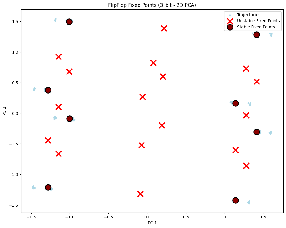
    # Visualize fixed points - 2D
    config_2d = PlotConfig(
        title=f"FlipFlop Fixed Points ({config_name} - 2D PCA)",
        xlabel="PC 1", ylabel="PC 2", figsize=(10, 8),
        show=True
    )
    plot_fixed_points_2d(unique_fps, hiddens_np, config=config_2d)

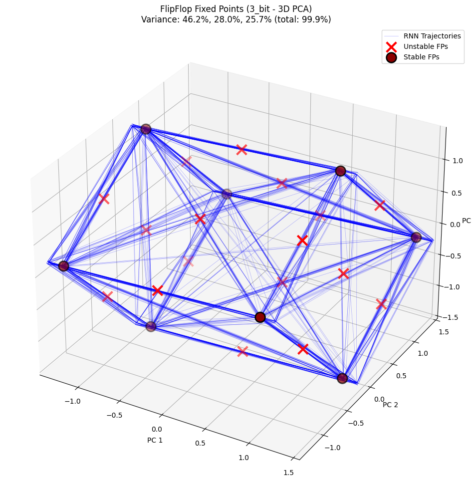
    # Visualize fixed points - 3D
    config_3d = PlotConfig(
        title=f"FlipFlop Fixed Points ({config_name} - 3D PCA)",
        figsize=(12, 10),
        show=True
    )
    plot_fixed_points_3d(
        unique_fps, hiddens_np, config=config_3d,
        plot_batch_idx=list(range(30)), plot_start_time=10
    )

print("\n--- Analysis complete ---")

--- Fixed Point Analysis Results ---

=== Fixed Points Summary ===
Number of fixed points: 25
State dimension: 4
Input dimension: 3

q values: min=0.00e+00, median=6.78e-19, max=9.87e-15
Iterations: min=384, median=384, max=384

Stable fixed points: 8 / 25

Detailed Fixed Point Information (Top 10):
#    q-value      Stability    Max |eig|
---------------------------------------------
1    1.78e-15     Stable       0.2418
2    0.00e+00     Stable       0.2308
3    0.00e+00     Stable       0.2291
4    6.78e-19     Unstable     1.7985
5    1.78e-15     Unstable     2.1942
6    0.00e+00     Stable       0.2417
7    0.00e+00     Stable       0.2435
8    0.00e+00     Stable       0.2291
9    0.00e+00     Stable       0.2436
10   1.78e-15     Stable       0.2307

  PCA explained variance: [0.46209928 0.27972662 0.25745255]
  Total variance explained: 99.93%

--- Analysis complete ---

5. Multi-Configuration Comparison: 2-bit, 3-bit, 4-bit

Below we will run all three configurations to demonstrate fixed point analysis results for tasks of different complexity.

Expected Results: - 2-bit: 4 stable fixed points (2² = 4 memory states) - 3-bit: 8 stable fixed points (2³ = 8 memory states) - 4-bit: 16 stable fixed points (2⁴ = 16 memory states)

import matplotlib.pyplot as plt

def run_flipflop_analysis(config_name, seed=42):
    """Run complete analysis pipeline for a single configuration"""
    config = TASK_CONFIGS[config_name]
    n_bits = config["n_bits"]
    n_hidden = config["n_hidden"]
    n_trials_train = config["n_trials_train"]
    n_inits = config["n_inits"]

    # Set random seeds
    np.random.seed(seed)
    random.seed(seed)

    print(f"\n{'='*60}")
    print(f"Configuration: {config_name} ({n_bits} bits, {n_hidden} hidden units)")
    print(f"{'='*60}")

    # Generate data
    data_gen = FlipFlopData(n_bits=n_bits, n_time=64, p=0.5, random_seed=seed)
    train_data = data_gen.generate_data(n_trials_train)
    valid_data = data_gen.generate_data(128)
    test_data = data_gen.generate_data(128)

    # Create and train model
    rnn = FlipFlopRNN(n_inputs=n_bits, n_hidden=n_hidden,
                      n_outputs=n_bits, rnn_type="tanh", seed=seed)

    checkpoint_path = f"flipflop_rnn_{config_name}_checkpoint.msgpack"
    if not load_checkpoint(rnn, checkpoint_path):
        print(f"Training model...")
        train_flipflop_rnn(rnn, train_data, valid_data,
                          learning_rate=0.08, batch_size=128,
                          max_epochs=500, min_loss=1e-4, print_every=50)
    else:
        print(f"Loaded model from checkpoint: {checkpoint_path}")

    # Get hidden state trajectory
    inputs_jax = jnp.array(test_data["inputs"])
    outputs, hiddens = rnn(inputs_jax)
    hiddens_np = np.array(hiddens)

    # Fixed point analysis
    finder = FixedPointFinder(
        rnn, method="joint", max_iters=5000, lr_init=0.02,
        tol_q=1e-4, final_q_threshold=1e-6, tol_unique=1e-2,
        do_compute_jacobians=True, do_decompose_jacobians=True,
        outlier_distance_scale=10.0, verbose=True, super_verbose=False,
    )

    constant_input = np.zeros((1, n_bits), dtype=np.float32)
    unique_fps, _ = finder.find_fixed_points(
        state_traj=hiddens_np, inputs=constant_input,
        n_inits=n_inits, noise_scale=0.4,
    )

    return unique_fps, hiddens_np, config_name

# Store results for all configurations
all_results = {}
for cfg in ["2_bit", "3_bit", "4_bit"]:
    unique_fps, hiddens_np, name = run_flipflop_analysis(cfg, seed=43)
    all_results[cfg] = {"fps": unique_fps, "hiddens": hiddens_np}

    # Print summary
    n_stable = np.sum(unique_fps.is_stable) if unique_fps.n > 0 else 0
    expected = 2 ** int(cfg[0])
    print(f"\nResults: Found {unique_fps.n} fixed points, {n_stable} stable (expected: {expected})")

============================================================
Configuration: 2_bit (2 bits, 3 hidden units)
============================================================
Training model...

======================================================================
Training FlipFlop RNN (Using brainpy optimizer)
======================================================================

Training parameters:
  Batch size: 128
  Learning rate:0.080000 (Fixed)
Epoch    0: train_loss = 0.933466, valid_loss = 0.676156
Epoch   50: train_loss = 0.000569, valid_loss = 0.000562
Epoch  100: train_loss = 0.000369, valid_loss = 0.000366
Epoch  150: train_loss = 0.000271, valid_loss = 0.000268
Epoch  200: train_loss = 0.000210, valid_loss = 0.000208
Epoch  250: train_loss = 0.000169, valid_loss = 0.000168
Epoch  300: train_loss = 0.000139, valid_loss = 0.000138
Epoch  350: train_loss = 0.000116, valid_loss = 0.000115

Reached target loss 1.00e-04 at epoch 395

======================================================================
Training Complete!
======================================================================
Final training loss: 0.000100
Final validation loss: 0.000099
Total epochs: 396

Searching for fixed points from 1024 initial states.

        Finding fixed points via joint optimization.

/var/folders/x0/_jqxxbbn0rsdn6b4h6fxbrjr0000gn/T/ipykernel_3897/1594189833.py:52: UserWarning: Joint optimization with n_inits=1024 may be inefficient and use excessive memory. Consider using sequential optimization or reducing n_inits.
  unique_fps, _ = finder.find_fixed_points(

        Optimization complete to desired tolerance.
                170 iters, q = 9.62e-08 +/- 2.84e-06, dq = 1.36e-07 +/- 4.32e-06, lr = 1.63e-02, avg iter time = 7.56e-03 sec
        Identified 9 unique fixed points.
        Computing recurrent Jacobian at 9 unique fixed points.
        Computing input Jacobian at 9 unique fixed points.
Decomposing 9 Jacobians...
Found 4 stable and 5 unstable fixed points.
        Applying final q-value filter (q < 1.0e-06)...
                9 high-quality fixed points remain.
        Fixed point finding complete.


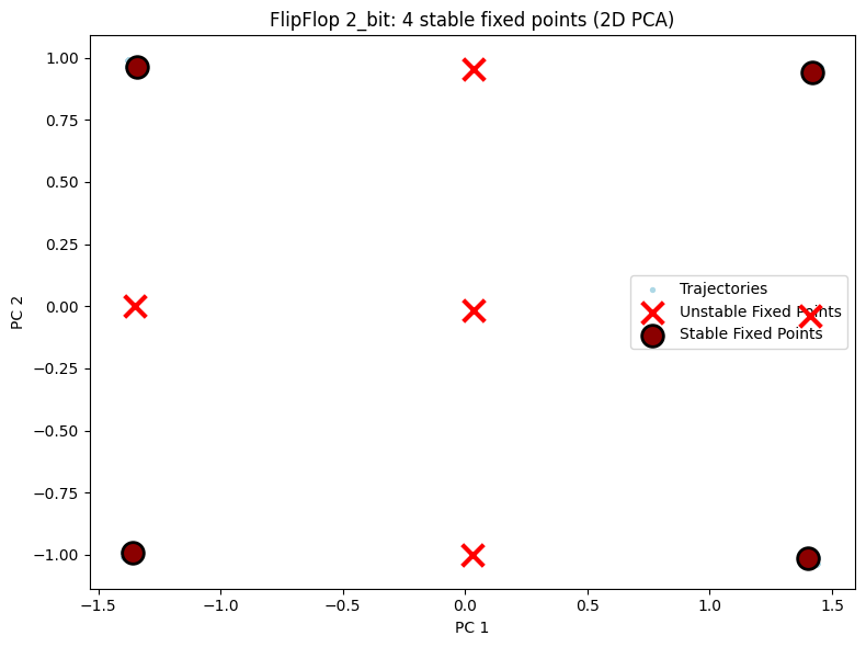
Results: Found 9 fixed points, 4 stable (expected: 4)

============================================================
Configuration: 3_bit (3 bits, 4 hidden units)
============================================================
Training model...

======================================================================
Training FlipFlop RNN (Using brainpy optimizer)
======================================================================

Training parameters:
  Batch size: 128
  Learning rate:0.080000 (Fixed)
Epoch    0: train_loss = 0.917904, valid_loss = 0.676378
Epoch   50: train_loss = 0.000278, valid_loss = 0.000279
Epoch  100: train_loss = 0.000161, valid_loss = 0.000163
Epoch  150: train_loss = 0.000116, valid_loss = 0.000117

Reached target loss 1.00e-04 at epoch 180

======================================================================
Training Complete!
======================================================================
Final training loss: 0.000100
Final validation loss: 0.000101
Total epochs: 181

Searching for fixed points from 1024 initial states.

        Finding fixed points via joint optimization.
        Optimization complete to desired tolerance.
                162 iters, q = 1.36e-07 +/- 3.03e-06, dq = 1.90e-08 +/- 4.74e-07, lr = 2.00e-02, avg iter time = 4.13e-03 sec
        Identified 27 unique fixed points.
        Computing recurrent Jacobian at 27 unique fixed points.
        Computing input Jacobian at 27 unique fixed points.
Decomposing 27 Jacobians...
Found 9 stable and 18 unstable fixed points.
        Applying final q-value filter (q < 1.0e-06)...
                Excluded 1 low-quality fixed points.
                26 high-quality fixed points remain.
        Fixed point finding complete.


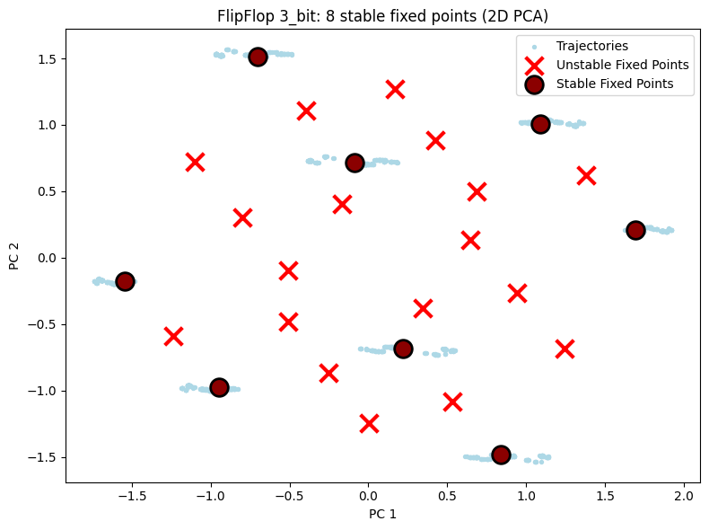
Results: Found 26 fixed points, 8 stable (expected: 8)

============================================================
Configuration: 4_bit (4 bits, 6 hidden units)
============================================================
Training model...

======================================================================
Training FlipFlop RNN (Using brainpy optimizer)
======================================================================

Training parameters:
  Batch size: 128
  Learning rate:0.080000 (Fixed)
Epoch    0: train_loss = 0.915913, valid_loss = 0.698172
Epoch   50: train_loss = 0.000216, valid_loss = 0.000215
Epoch  100: train_loss = 0.000131, valid_loss = 0.000130

Reached target loss 1.00e-04 at epoch 140

======================================================================
Training Complete!
======================================================================
Final training loss: 0.000100
Final validation loss: 0.000100
Total epochs: 141

Searching for fixed points from 1024 initial states.

        Finding fixed points via joint optimization.
        Optimization complete to desired tolerance.
                333 iters, q = 4.02e-07 +/- 4.73e-06, dq = 1.24e-08 +/- 1.45e-07, lr = 2.00e-02, avg iter time = 5.46e-03 sec
        Identified 74 unique fixed points.
        Computing recurrent Jacobian at 74 unique fixed points.
        Computing input Jacobian at 74 unique fixed points.
Decomposing 74 Jacobians...
Found 22 stable and 52 unstable fixed points.
        Applying final q-value filter (q < 1.0e-06)...
                Excluded 7 low-quality fixed points.
                67 high-quality fixed points remain.
        Fixed point finding complete.


Results: Found 67 fixed points, 16 stable (expected: 16)

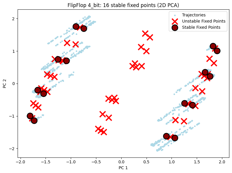
5.1 2D Visualization Comparison

Shows 2D PCA projections for all three configurations. You can visually see the fixed points increase as task complexity grows.

# 2D visualization - display each configuration separately
for cfg in ["2_bit", "3_bit", "4_bit"]:
    result = all_results[cfg]
    unique_fps = result["fps"]
    hiddens_np = result["hiddens"]

    n_bits = int(cfg[0])
    n_stable = np.sum(unique_fps.is_stable) if unique_fps.n > 0 else 0

    config_2d = PlotConfig(
        title=f"FlipFlop {cfg}: {n_stable} stable fixed points (2D PCA)",
        xlabel="PC 1", ylabel="PC 2",
        figsize=(8, 6),
        show=True
    )

    plot_fixed_points_2d(unique_fps, hiddens_np, config=config_2d)

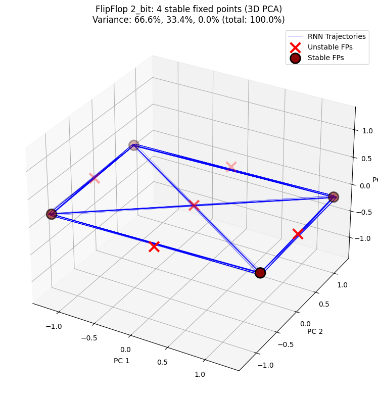
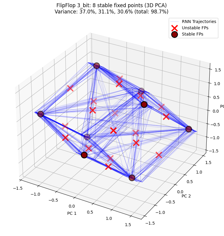
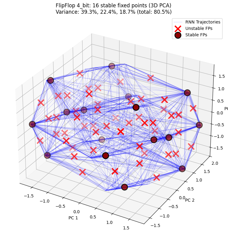
5.2 3D Visualization Comparison

3D PCA projection shows the distribution of hidden state trajectories and fixed points in three-dimensional space, providing a clearer view of the RNN’s dynamical structure.

# 3D visualization - display each configuration separately
for cfg in ["2_bit", "3_bit", "4_bit"]:
    result = all_results[cfg]
    unique_fps = result["fps"]
    hiddens_np = result["hiddens"]

    n_bits = int(cfg[0])
    n_stable = np.sum(unique_fps.is_stable) if unique_fps.n > 0 else 0

    config_3d = PlotConfig(
        title=f"FlipFlop {cfg}: {n_stable} stable fixed points (3D PCA)",
        figsize=(10, 8),
        show=True
    )

    plot_fixed_points_3d(
        unique_fps, hiddens_np, config=config_3d,
        plot_batch_idx=list(range(20)), plot_start_time=10
    )

  PCA explained variance: [6.6613883e-01 3.3384740e-01 1.3795699e-05]
  Total variance explained: 100.00%

  PCA explained variance: [0.37013304 0.3110425  0.3062212 ]
  Total variance explained: 98.74%

  PCA explained variance: [0.3934802  0.22392422 0.18720938]
  Total variance explained: 80.46%

6. Summary

This tutorial demonstrated how to use FixedPointFinder to analyze the dynamical structure of an RNN:

1. FlipFlop Task: The RNN must remember states across multiple binary channels

2. Fixed Point Analysis: Find the stable states the RNN uses for “memory” [29, 30]

3. Visualization: Use PCA dimensionality reduction to show the distribution of fixed points in hidden state space

Key Findings: - For an N-bit task, the RNN learns to create 2^N stable fixed points - These fixed points correspond to different combinations of memory states - Fixed point analysis is a powerful tool for understanding the internal computational mechanisms of RNNs