如何生成任务数据?
目标: 通过本指南,您将能够为 CANN 仿真生成任务输入。
预计阅读时间: 10 分钟
介绍
CANN 模型需要输入刺激来模拟真实行为——跟踪移动目标、编码空间位置或响应群体编码信号。与其手动创建这些输入,任务 API 为常见实验范式提供了现成的生成器。
本指南将向您展示如何:
创建平滑跟踪任务
生成任务数据
理解任务数据结构
在仿真中使用任务数据
什么是任务?
任务 是为 CANN 模型生成时变输入刺激的对象。它们处理以下复杂性:
创建生物学上真实的输入模式
管理时间和持续时间
格式化数据以实现高效的仿真循环
跟踪元数据(例如目标位置、速度)
关键原则: 任务 生成输入 → 模型在仿真循环中 消耗输入 。
创建平滑跟踪任务
最常见的任务是 平滑跟踪 ,其中刺激在神经群体中平滑移动:
[1]:
import brainpy.math as bm
from canns.models.basic import CANN1D
from canns.task.tracking import SmoothTracking1D
import jax

# Set up environment and model (from previous guide)
bm.set_dt(0.1)
cann = CANN1D(num=512)

# Create a smooth tracking task
task = SmoothTracking1D(
    cann_instance=cann,                # Link to the CANN model
    Iext=(1.0, 0.75, 2.0, 1.75, 3.0),  # External input positions (in radians)
    duration=(10.0, 10.0, 10.0, 10.0), # Duration at each position (ms)
    time_step=bm.get_dt()  # Simulation time step
)
发生了什么:
cann_instance: 任务需要模型实例来访问其get_stimulus_by_pos()方法,该方法为给定位置生成空间定位的输入模式。任务还使用模型的结构(神经元位置、网络大小)来创建适当的刺激。Iext: 刺激将出现的目标位置序列(弧度制,从 -π 到 π)duration: 刺激在每个位置停留多长时间(毫秒)time_step: 应与模型的dt匹配以保持同步
重要:CANN 模型必须提供一个 get_stimulus_by_pos(position) 方法,该方法返回给定空间位置的输入模式。任务调用此方法来生成数据。
生成数据
任务创建后,生成实际的输入数组:
[2]:
# Generate all task data
task.get_data()
<SmoothTracking1D> Generating Task data: 400it [00:00, 1593.79it/s]
此方法会预计算整个仿真的所有输入刺激。数据存储在 task.data 中。
理解任务数据结构
让我们检查任务生成的内容:
[3]:
print(f"Data shape: {task.data.shape}")
print(f"Number of time steps: {task.run_steps.shape[0]}")
print(f"Time step size: {task.time_step} ms")
print(f"Total simulation time: {task.run_steps.shape[0] * task.time_step} ms")
Data shape: (400, 512)
Number of time steps: 400
Time step size: 0.1 ms
Total simulation time: 40.0 ms
[4]:
from canns.analyzer.visualization import PlotConfigs, energy_landscape_1d_static

# Create configuration for static plot
config = PlotConfigs.energy_landscape_1d_static(
    time_steps_per_second=100,
    title='Input Stimulus at t=50',
    xlabel='Position (rad)',
    ylabel='Input Strength',
    show=True
)

# Plot input at time step 50
energy_landscape_1d_static(
    data_sets={'Stimulus': (cann.x, task.data[50])},
    config=config
)
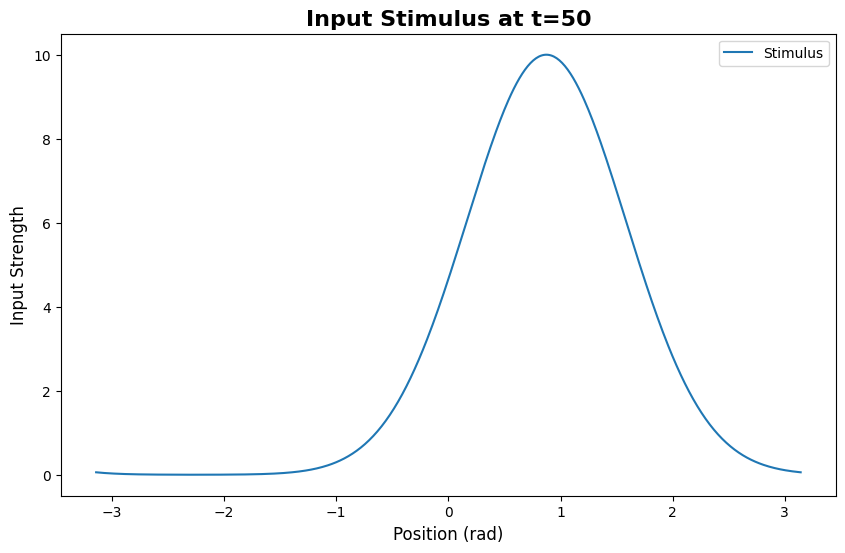
[4]:
(<Figure size 1000x600 with 1 Axes>,
 <Axes: title={'center': 'Input Stimulus at t=50'}, xlabel='Position (rad)', ylabel='Input Strength'>)
您将看到一个以 Iext 指定位置之一为中心的高斯形波包。
在仿真中使用任务数据
现在将任务数据连接到您的模型仿真:
[5]:
def run_step(t, stimulus):
    """Simulation step function."""
    cann(stimulus)  # Feed stimulus to model
    return cann.u.value, cann.r.value  # Return synaptic input and activity

# Run the simulation with task data
us, rs = bm.for_loop(
    run_step,
    operands=(task.run_steps, task.data),
    progress_bar=10
)

print(f"Synaptic input shape: {us.shape}")   # (400, 512)
print(f"Neural activity shape: {rs.shape}")  # (400, 512)
Synaptic input shape: (400, 512)
Neural activity shape: (400, 512)
工作流程:
task.data为每个时间步提供刺激for_loop遍历时间步在每一步中,刺激被传递给
run_step模型更新其状态并返回结果
所有结果被收集到数组(
us、rs)中
完整工作示例
以下是从模型创建到任务驱动仿真的完整流程:
[6]:
import brainpy.math as bm  # :cite:p:`wang2023brainpy`
from canns.models.basic import CANN1D
from canns.task.tracking import SmoothTracking1D

# 1. Setup
bm.set_dt(0.1)

# 2. Create model (auto-initializes)
cann = CANN1D(num=512)

# 3. Create task
task = SmoothTracking1D(
    cann_instance=cann,
    Iext=(1.0, 0.75, 2.0, 1.75, 3.0),
    duration=(10.0, 10.0, 10.0, 10.0),
    time_step=bm.get_dt(),
)
task.get_data()

# 4. Run simulation
def run_step(t, stimulus):
    cann(stimulus)
    return cann.u.value, cann.r.value

us, rs = bm.for_loop(
    run_step,
    operands=(task.run_steps, task.data),
    progress_bar=10
)

print("Simulation complete!")
print(f"Captured {us.shape[0]} time steps of activity")
<SmoothTracking1D> Generating Task data: 400it [00:00, 3246.41it/s]
Simulation complete!
Captured 400 time steps of activity
探索任务参数
SmoothTracking1D 非常灵活。尝试不同的配置:
示例 1: 快速追踪
[7]:
task_fast = SmoothTracking1D(
    cann_instance=cann,
    Iext=(0.0, 1.0, 2.0),
    duration=(5.0, 5.0),  # Shorter durations = faster transitions
    time_step=0.1
)
示例 2: 更多位置
[9]:
import jax.numpy as jnp

# Track across 10 evenly spaced positions
positions = jnp.linspace(-3.0, 3.0, 10)
durations = [8.0] * 9

task_dense = SmoothTracking1D(
    cann_instance=cann,
    Iext=tuple(positions),
    duration=tuple(durations),
    time_step=0.1
)
示例 3: 可变持续时间
[10]:
# Different durations for each position
task_variable = SmoothTracking1D(
    cann_instance=cann,
    Iext=(0.0, 1.5, -1.0, 2.0),
    duration=(15.0, 5.0, 10.0),  # Stay longer at first position
    time_step=0.1
)
其他任务类型
虽然本指南重点关注 SmoothTracking1D,但该库还包含其他任务生成器:
SmoothTracking2D: 2D 空间追踪PopulationCoding: 群体编码输入ClosedLoopNavigation: 带反馈的交互式导航OpenLoopNavigation: 预定义轨迹
所有任务都遵循相同的模式:
使用参数创建任务
调用
task.get_data()在仿真循环中使用
task.data
我们将在”详细信息”部分探讨这些任务。
常见问题
问: 生成任务数据后,我可以修改它吗?
可以!task.data 是一个您可以操作的 JAX 数组:
[11]:
task.get_data()
# Add noise to all inputs
task.data = task.data + 0.1 * jax.random.normal(jax.random.PRNGKey(0), task.data.shape)
<SmoothTracking1D> Generating Task data: 400it [00:00, 9170.08it/s]
问: 如果我想要自定义输入模式怎么办?
您可以创建任务作为模板并修改它们,或手动生成输入:
[12]:
import jax.numpy as jnp

# Create custom input sequence
custom_data = jnp.zeros((100, 512))
for t in range(100):
    position = jnp.sin(t * 0.1)  # Sinusoidal movement
    custom_data = custom_data.at[t].set(
        jnp.exp(-0.5 * (cann.x - position)**2 / 0.3**2)
    )
问: 我每次都需要调用 ``get_data()`` 吗?
每个任务实例只需调用一次。数据被缓存:
[ ]:
task.get_data()  # Generates data
# ... use task.data in simulations

# If you change parameters, recreate the task
task_new = SmoothTracking1D(...)
task_new.get_data()
后续步骤
现在您已经可以生成任务数据,接下来可以:
分析 CANN 模型动力学——可视化能量景观、波包追踪等
探索任务生成器——了解所有可用的任务类型及其用例
完整任务 API 参考——所有任务参数和方法的完整文档
有疑问?打开 `GitHub Discussion <https://github.com/routhleck/canns/discussions>`_.