How to Analyze CANN Models?
Goal: By the end of this guide, you’ll be able to visualize CANN dynamics using energy landscape plots.
Estimated Reading Time: 12 minutes
Introduction
After running a CANN simulation, you need to visualize the results to understand the network’s behavior. Did the bump form correctly? Is it tracking the stimulus? Is the activity stable?
The Analyzer module provides visualization tools specifically designed for CANN dynamics. This guide focuses on the most essential visualization: energy landscape plots.
You’ll learn to:
What is an Energy Landscape?
An energy landscape shows how neural activity evolves over time:
X-axis: Neuron position (for 1D CANNs, this is angular position from -π to π)
Y-axis: Neural activity or synaptic input
Animation: Time evolution of the activity pattern
This visualization is perfect for observing:
Bump formation: Does a localized activity bump emerge?
Tracking: Does the bump follow external stimuli?
Stability: Does the bump maintain its shape and position?
The PlotConfig System
Before diving into examples, understand the visualization architecture.
The library uses PlotConfig dataclasses to manage plot settings. This provides:
Consistency: Same parameters across different plot types
Reusability: Save and reuse configurations
Type safety: Clear parameter names and validation
[ ]:
from canns.analyzer.visualization import PlotConfigs
# Create a configuration for animation
config = PlotConfigs.energy_landscape_1d_animation(
time_steps_per_second=100, # Simulation speed (100 steps/sec)
fps=20, # Animation frame rate
title='My CANN Simulation',
xlabel='Position (rad)',
ylabel='Activity',
save_path='output.gif',
show=False # Don't display, just save
)
Why PlotConfig? Instead of passing 10+ arguments to a function, you configure once and reuse. This becomes especially valuable when creating multiple similar plots.
Complete Workflow: From Model to Visualization
Let’s build a full example—creating, simulating, and visualizing a CANN:
[1]:
import brainpy.math as bm # :cite:p:`wang2023brainpy`
from canns.models.basic import CANN1D
from canns.task.tracking import SmoothTracking1D
from canns.analyzer.visualization import PlotConfigs, energy_landscape_1d_animation
# 1. Setup
bm.set_dt(0.1)
# 2. Create model (auto-initializes)
cann = CANN1D(num=512)
# 3. Create task
task = SmoothTracking1D(
cann_instance=cann,
Iext=(1.0, 0.75, 2.0, 1.75, 3.0),
duration=(10.0, 10.0, 10.0, 10.0),
time_step=bm.get_dt(),
)
task.get_data()
# 4. Run simulation
def run_step(t, inputs):
cann(inputs)
return cann.u.value, cann.r.value
us, rs = bm.for_loop(
run_step,
operands=(task.run_steps, task.data),
progress_bar=10
)
print("Simulation complete! Now visualizing...")
# 5. Create visualization config
config = PlotConfigs.energy_landscape_1d_animation(
time_steps_per_second=100,
fps=20,
title='CANN1D Smooth Tracking',
xlabel='Position (rad)',
ylabel='Activity',
repeat=True,
show=True,
)
# 6. Generate animation
energy_landscape_1d_animation(
data_sets={
'u': (cann.x, us), # Synaptic input over time
'Iext': (cann.x, task.data) # External stimulus
},
config=config
)
<SmoothTracking1D> Generating Task data: 400it [00:00, 1848.42it/s]
Simulation complete! Now visualizing...
What’s happening in step 6:
data_sets: Dictionary mapping labels to(positions, data)tuplescann.x: Neuron positions (x-axis values)us: Activity over time (shape[time_steps, num_neurons])task.data: Original input stimuli for comparison
The animation will show two curves:
Blue (u): The CANN’s internal activity
Orange (Iext): The external input stimulus
You’ll see the activity bump tracking the moving stimulus!
Static Plots for Quick Inspection
For quick checks without generating full animations:
[2]:
from canns.analyzer.visualization import PlotConfigs, energy_landscape_1d_static
# Configuration for static plot
config_static = PlotConfigs.energy_landscape_1d_static(
time_steps_per_second=100,
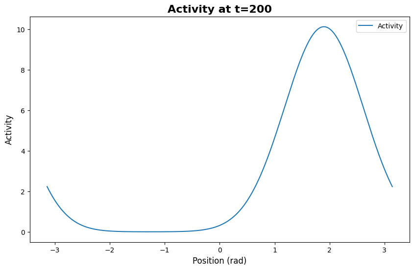
title='Activity at t=200',
xlabel='Position (rad)',
ylabel='Activity',
save_path='snapshot_t200.png',
show=True # Display the plot
)
# Plot activity at specific time step (e.g., t=200)
energy_landscape_1d_static(
data_sets={'Activity': (cann.x, us[200])}, # Single time step
config=config_static
)
Plot saved to: snapshot_t200.png
[2]:
(<Figure size 1000x600 with 1 Axes>,
<Axes: title={'center': 'Activity at t=200'}, xlabel='Position (rad)', ylabel='Activity'>)
Use case: Quickly check if the model reached a stable state at a particular time.
Comparing Models: CANN vs. CANN-SFA
This section compares standard CANN with CANN-SFA [9, 10] models.
One powerful visualization technique is comparing different models side-by-side. Let’s compare a standard CANN with a CANN that includes Spike Frequency Adaptation (SFA):
[4]:
import brainpy.math as bm # :cite:p:`wang2023brainpy`
from canns.models.basic import CANN1D, CANN1D_SFA # SFA: :cite:p:`mi2014spike,li2025dynamics`
from canns.task.tracking import SmoothTracking1D
from canns.analyzer.visualization import PlotConfigs, energy_landscape_1d_animation
bm.set_dt(0.1)
# Create two models (auto-initialize)
cann_standard = CANN1D(num=512)
cann_sfa = CANN1D_SFA(num=512, tau_v=50.0) # SFA with adaptation time constant
# Same task for both
task = SmoothTracking1D(
cann_instance=cann_standard, # Use one model as reference
Iext=(1.0, 0.75, 2.0, 1.75, 3.0),
duration=(10.0, 10.0, 10.0, 10.0),
time_step=0.1,
)
task.get_data()
# Simulate standard CANN
def step_standard(t, inputs):
cann_standard(inputs)
return cann_standard.u.value
us_standard = bm.for_loop(
step_standard,
operands=(task.run_steps, task.data),
progress_bar=10
)
# Simulate CANN-SFA
def step_sfa(t, inputs):
cann_sfa(inputs)
return cann_sfa.u.value
us_sfa = bm.for_loop(
step_sfa,
operands=(task.run_steps, task.data),
progress_bar=10
)
# Visualize both in one animation
config_comparison = PlotConfigs.energy_landscape_1d_animation(
time_steps_per_second=100,
fps=20,
title='CANN vs CANN-SFA: Oscillatory Tracking',
xlabel='Position (rad)',
ylabel='Activity',
repeat=True,
show=True,
)
energy_landscape_1d_animation(
data_sets={
'CANN (Standard)': (cann_standard.x, us_standard),
'CANN-SFA': (cann_sfa.x, us_sfa),
'Input': (cann_standard.x, task.data)
},
config=config_comparison
)
<SmoothTracking1D> Generating Task data: 400it [00:00, 9277.33it/s]
What you’ll observe:
Standard CANN: Bump follows input closely
CANN-SFA: Bump may show oscillatory behavior or delayed tracking due to adaptation
Insight: SFA introduces history-dependent dynamics—visible as different tracking patterns
This comparison helps you understand how model variants behave differently under the same conditions.
Customizing Visualizations
Adjusting Animation Speed
[ ]:
config_slow = PlotConfigs.energy_landscape_1d_animation(
time_steps_per_second=50, # Show 50 steps per second (slower)
fps=10, # 10 frames per second (smoother)
...
)
Rule of thumb: time_steps_per_second / fps = steps per frame
Higher ratio = faster animation
Lower ratio = slower, more detailed animation
Changing Appearance
[ ]:
config_styled = PlotConfigs.energy_landscape_1d_animation(
figsize=(10, 4), # Wider figure
title='Custom Styled Plot',
xlabel='Angular Position',
ylabel='Firing Rate (Hz)',
title_fontsize=14,
save_path='styled_output.gif',
show=False
)
Saving vs. Displaying
[ ]:
# Save only (for batch processing)
config_save = PlotConfigs.energy_landscape_1d_animation(
save_path='output.gif',
show=False
)
# Display only (for interactive exploration)
config_display = PlotConfigs.energy_landscape_1d_animation(
save_path=None,
show=True
)
# Both
config_both = PlotConfigs.energy_landscape_1d_animation(
save_path='output.gif',
show=True
)
More Analysis Tools
This guide focuses on energy landscapes, but the analyzer module includes many other tools:
Tuning curves: Neuron selectivity plots
Firing fields: Spatial response maps
Bump fitting: Extract bump position and width
Spike plots: Raster plots for spike-based models
These are covered in detail in the Full Details: Model Analyzer section.
Next Steps
Now that you can visualize CANN dynamics, you’re ready to:
Analyze experimental data—Apply similar techniques to real neural recordings
Explore Model Analyzer—Learn about all available analysis methods
Full Visualization API—Complete reference for PlotConfig and all plot functions
Questions? Check the PlotConfig Guide or GitHub Discussions.