Tutorial 6: Hierarchical Path Integration Network

Tutorial Info

Reading Time: 35-40 minutes

Difficulty: Advanced

Prerequisites: Tutorial 1: Building and Using CANN Models

This tutorial introduces hierarchical path integration networks, which combine multi-scale grid cells [2] for robust spatial navigation in large environments.

Important

Reference Publication

This tutorial implements the model from: Chu et al. (2025)—“Localized Space Coding and Phase Coding Complement Each Other to Achieve Robust and Efficient Spatial Representation” [19]

For detailed theoretical background and experimental validation, please refer to the original paper.

1. Introduction to Hierarchical Path Integration

1.1 What is Hierarchical Path Integration?

Path integration is the ability to track position by integrating self-motion signals (velocity) over time. Hierarchical path integration [4, 19, 28] uses multiple grid cell [2] modules operating at different spatial scales to achieve:

• Multi-scale representation: Coarse scales for large spaces, fine scales for precision

• Error correction: Multiple scales provide redundancy against drift

• Efficient coding: Different modules tile space at different resolutions

1.2 Biological Inspiration

In the mammalian brain:

• Grid cells [2] in medial entorhinal cortex fire at regular spatial intervals forming hexagonal patterns

• Multiple modules exist with different grid spacings (30cm to several meters)

• Band cells integrate velocity along preferred directions

• Place cells [1] in hippocampus receive convergent input from grid cells, forming localized spatial representations [19]

1.3 Key Components

The hierarchical network consists of:

1. Band Cells—Velocity integrators along specific orientations (0°, 60°, 120°)

2. Grid Cells [2]—2D continuous attractors [5, 28] forming hexagonal patterns

3. Place Cells [1]—Readout layer combining information from all modules

4. Multi-Module Architecture—Multiple grid modules with different spacings

2. Model Architecture

2.1 Component Overview

from canns.models.basic import HierarchicalNetwork

# Create hierarchical network with 5 modules
hierarchical_net = HierarchicalNetwork(
    num_module=5,        # Number of grid modules (different scales)
    num_place=30,        # Place cells per dimension (30x30 = 900 total)
    spacing_min=2.0,     # Smallest grid spacing
    spacing_max=5.0,     # Largest grid spacing
    module_angle=0.0     # Base orientation angle
)

2.2 Key Parameters

Parameter	Type	Description
num_module	int	Number of grid modules with different scales
num_place	int	Place cells per spatial dimension
spacing_min	float	Minimum grid spacing (finest scale)
spacing_max	float	Maximum grid spacing (coarsest scale)
module_angle	float	Base orientation for grid modules

Parameter Guidelines:

• num_module=5: Good balance between coverage and computation

• num_place=30: Provides 900 place cells for 5x5m environment

• Spacing range should match environment size (larger spaces need larger spacing_max)

2.3 Internal Structure

Each module contains:

• 3 BandCell networks at 0°, 60°, 120° orientations

• 1 GridCell network combining band cell outputs

• Connections project to shared place cell population

3. Complete Example: Multi-Scale Navigation

3.1 Setup and Task Creation

import brainpy.math as bm
import numpy as np
from canns.models.basic import HierarchicalNetwork
from canns.task.open_loop_navigation import OpenLoopNavigationTask

# Setup environment
bm.set_dt(0.05)

# Create navigation task (5m x 5m environment)
task = OpenLoopNavigationTask(
    width=5.0,           # Environment width (meters)
    height=5.0,          # Environment height (meters)
    speed_mean=0.04,     # Mean speed (m/step)
    speed_std=0.016,     # Speed standard deviation
    duration=50000.0,    # Simulation duration (steps)
    dt=0.05,             # Time step
    start_pos=(2.5, 2.5), # Start at center
    progress_bar=True
)

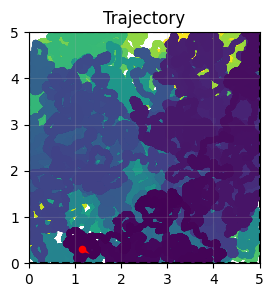
# Generate trajectory data
task.get_data()

print(f"Trajectory: {task.data.position.shape[0]} steps")
print(f"Environment: {task.width}m x {task.height}m")
task.show_data()

<OpenLoopNavigationTask>Generating Task data: 100%|██████████| 1000000/1000000 [00:00<00:00, 1468708.52it/s]

Trajectory: 1000000 steps
Environment: 5.0m x 5.0m

3.2 Create Hierarchical Network

# Create hierarchical network
hierarchical_net = HierarchicalNetwork(
    num_module=5,         # 5 different spatial scales
    num_place=30,         # 30x30 place cell grid
    spacing_min=2.0,      # Finest grid scale
    spacing_max=5.0,      # Coarsest grid scale
)

3.3 Initialization Phase

Critical Step: Initialize the network with strong location input to set initial position.

def initialize(t, input_strength):
    """Initialize network with location input"""
    hierarchical_net(
        velocity=bm.zeros(2,),        # No velocity during init
        loc=task.data.position[0],        # Starting position
        loc_input_stre=input_strength,    # Input strength
    )

# Create initialization schedule
init_time = 500
indices = np.arange(init_time)
input_strength = np.zeros(init_time)
input_strength[:400] = 100.0  # Strong input for first 400 steps

# Run initialization
bm.for_loop(
    initialize,
    operands=(bm.asarray(indices), bm.asarray(input_strength)),
    progress_bar=10,
)

print("Initialization complete")

Running for 500 iterations: 100%|██████████| 500/500 [00:00<00:00, 1896.23it/s]

Initialization complete

Why initialization matters:

• Sets all grid modules to consistent starting state

• Strong location input (100.0) anchors the network

• Without proper init, modules may start desynchronized

3.4 Main Simulation Loop

def run_step(t, vel, loc):
    """Single simulation step with velocity input"""
    hierarchical_net(
        velocity=vel,           # Current velocity
        loc=loc,                # Current position (for reference)
        loc_input_stre=0.0      # No location input during navigation
    )

    # Extract firing rates from all layers
    band_x_r = hierarchical_net.band_x_fr.value   # X-direction band cells
    band_y_r = hierarchical_net.band_y_fr.value   # Y-direction band cells
    grid_r = hierarchical_net.grid_fr.value       # Grid cells
    place_r = hierarchical_net.place_fr.value     # Place cells

    return band_x_r, band_y_r, grid_r, place_r

# Get trajectory data
total_time = task.data.velocity.shape[0]
indices = np.arange(total_time)

# Run simulation
print("Running main simulation...")
band_x_r, band_y_r, grid_r, place_r = bm.for_loop(
    run_step,
    operands=(
        bm.asarray(indices),
        bm.asarray(task.data.velocity),
        bm.asarray(task.data.position)
    ),
    progress_bar=10000,
)

print(f"Simulation complete!")
print(f"Band X cells: {band_x_r.shape}")
print(f"Band Y cells: {band_y_r.shape}")
print(f"Grid cells: {grid_r.shape}")
print(f"Place cells: {place_r.shape}")

Running main simulation...

Running for 1,000,000 iterations: 100%|██████████| 1000000/1000000 [07:18<00:00, 2278.48it/s]

Simulation complete!
Band X cells: (1000000, 5, 180)
Band Y cells: (1000000, 5, 180)
Grid cells: (1000000, 5, 400)
Place cells: (1000000, 900)

Understanding the outputs:

• band_x_r: Shape (T, num_module, num_cells) - Band cells for X components

• band_y_r: Shape (T, num_module, num_cells) - Band cells for Y components

• grid_r: Shape (T, num_module, num_gc_x, num_gc_y) - Grid cell activities

• place_r: Shape (T, num_place, num_place) - Place cell responses

4. Visualization and Analysis

4.1 Computing Firing Fields

Firing fields show where each neuron is active in the environment:

from canns.analyzer.metrics.spatial_metrics import compute_firing_field, gaussian_smooth_heatmaps
from canns.analyzer.visualization import PlotConfig, plot_firing_field_heatmap

# Prepare data
loc = np.array(task.data.position)
width = 5
height = 5
M = int(width * 10)
K = int(height * 10)

T = grid_r.shape[0]

# Reshape arrays for firing field computation
grid_r = grid_r.reshape(T, -1)
band_x_r = band_x_r.reshape(T, -1)
band_y_r = band_y_r.reshape(T, -1)
place_r = place_r.reshape(T, -1)

# Compute firing fields
print("Computing firing fields...")
heatmaps_grid = compute_firing_field(np.array(grid_r), loc, width, height, M, K)
heatmaps_band_x = compute_firing_field(np.array(band_x_r), loc, width, height, M, K)
heatmaps_band_y = compute_firing_field(np.array(band_y_r), loc, width, height, M, K)
heatmaps_place = compute_firing_field(np.array(place_r), loc, width, height, M, K)

# Apply Gaussian smoothing
heatmaps_grid = gaussian_smooth_heatmaps(heatmaps_grid)
heatmaps_band_x = gaussian_smooth_heatmaps(heatmaps_band_x)
heatmaps_band_y = gaussian_smooth_heatmaps(heatmaps_band_y)
heatmaps_place = gaussian_smooth_heatmaps(heatmaps_place)

print(f"Firing fields computed: {heatmaps_grid.shape}")

Computing firing fields...
Firing fields computed: (2000, 50, 50)

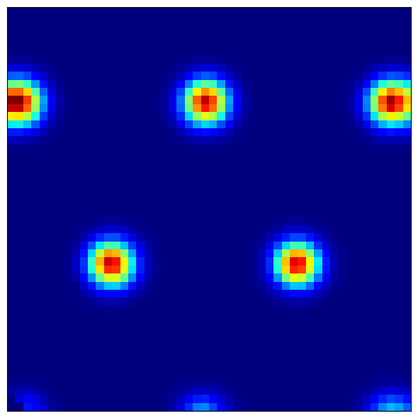
4.2 Visualizing Grid Cell Patterns

Grid cells show characteristic hexagonal firing patterns:

# Reshape to separate modules
heatmaps_grid = heatmaps_grid.reshape(5, -1, M, K)  # (modules, cells, x, y)

# Visualize a grid cell from module 0
module_idx = 0
cell_idx = 42

config = PlotConfig(
    figsize=(6, 6),
    title=f'Grid Cell - Module {module_idx}, Cell {cell_idx}',
    xlabel='X Position (m)',
    ylabel='Y Position (m)',
    show=True,
    save_path=None
)

plot_firing_field_heatmap(
    heatmaps_grid[module_idx, cell_idx],
    config=config
)

(<Figure size 600x600 with 1 Axes>, <Axes: >)

What to observe:

• Module 0 (finest scale): Small, tightly packed hexagons

• Module 4 (coarsest scale): Large, widely spaced hexagons

• Regular spacing: Grid vertices form equilateral triangles

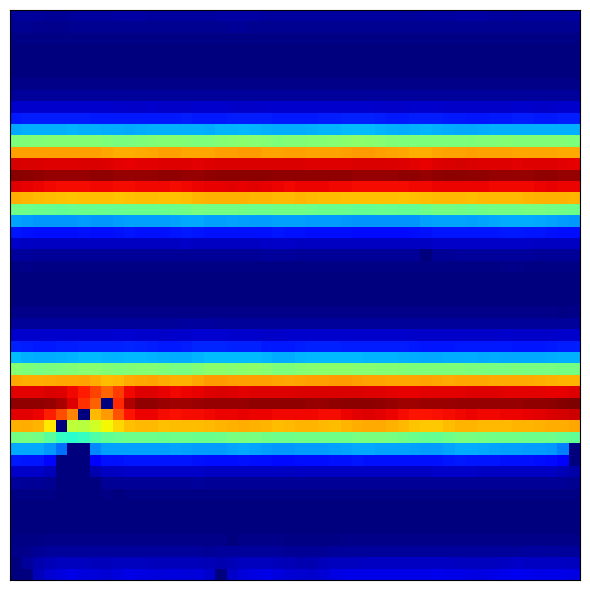
4.3 Visualizing Band Cell Patterns

Band cells show stripe-like patterns along their preferred orientation:

# Reshape band cells
heatmaps_band_x = heatmaps_band_x.reshape(5, -1, M, K)

# Visualize a band cell
config = PlotConfig(
    figsize=(6, 6),
    title=f'Band Cell X - Module {module_idx}, Cell {cell_idx}',
    xlabel='X Position (m)',
    ylabel='Y Position (m)',
    show=True,
    save_path=None
)

plot_firing_field_heatmap(
    heatmaps_band_x[module_idx, cell_idx],
    config=config
)

(<Figure size 600x600 with 1 Axes>, <Axes: >)

Expected patterns:

• Parallel stripes perpendicular to preferred direction

• Different cells have different stripe spacings (phase offsets)

• Multiple modules show different scales of striping

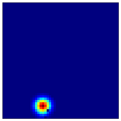
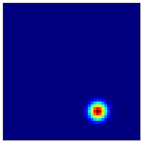
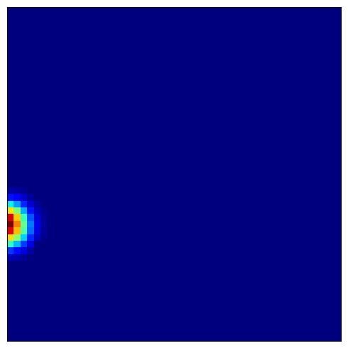
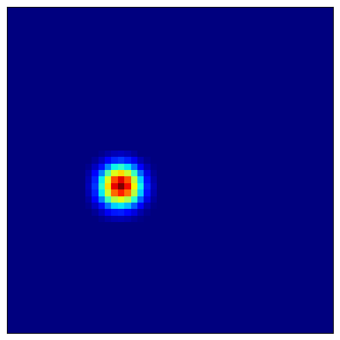
4.4 Visualizing Place Cell Fields

Place cells combine grid cell inputs to form localized firing fields:

# Visualize several place cells
for place_idx in [100, 200, 300, 400]:
    config = PlotConfig(
        figsize=(5, 5),
        title=f'Place Cell {place_idx}',
        xlabel='X Position (m)',
        ylabel='Y Position (m)',
        show=True,
        save_path=None
    )

    plot_firing_field_heatmap(
        heatmaps_place[place_idx],
        config=config
    )

5. Next Steps

Congratulations! You’ve completed the hierarchical path integration tutorial. You now understand:

• How multi-scale grid cell modules provide robust spatial coding

• The architecture combining band cells, grid cells, and place cells

• How to initialize hierarchical networks properly

• How to visualize firing fields across different spatial scales

What You’ve Learned

Hierarchical Architecture

You understand how multiple grid modules at different scales combine to create a robust spatial representation.

Multi-Scale Coding

You’ve seen how coarse scales provide large-scale coverage while fine scales provide precision.

Network Initialization

You know the critical importance of proper initialization with location input before running path integration.

Biological Realism

You’ve implemented a model that matches the organization of the mammalian entorhinal-hippocampal system [2, 19].

Continue Learning

Explore related advanced topics:

• Tutorial 7: Theta Sweep HD-Grid System - Learn theta-modulated systems combining head direction and grid cells

• Tutorial 8: Theta Sweep Place Cell Network - Understand place cells in complex environments with geodesic distances

Or explore other scenarios:

• Scenario 2: Data Analysis - Compare model predictions with experimental data

• Scenario 3: Brain-Inspired Learning - Train spatial memory systems

• Scenario 4: Pipeline - High-level pipeline tools for complete workflows

Key Takeaways

1. Multi-scale representation - Different grid spacings provide complementary information about position

2. Initialization matters - Strong location input is required to synchronize all modules

3. Band cells are building blocks - Grid cells emerge from combining band cell modules at different orientations

4. Place cells integrate - Place cells form localized fields by combining grid cell inputs

Advanced Topics

Error Correction

Multiple scales allow the network to correct accumulated drift errors. Fine scales detect small errors, coarse scales provide global reference.

Scaling Properties

Grid spacing typically follows a geometric progression (e.g., 2.0, 2.5, 3.1, 3.9, 4.9 meters for 5 modules).

Biological Parameters

Real grid cells have spacings from ~30cm to several meters. Adjust spacing_min and spacing_max to match experimental data.

Place Field Formation

Place cells can develop multiple firing fields in large environments due to grid cell periodicity.

Parameter Tuning Guidelines

For hierarchical networks:

• num_module=5-7: Good balance between coverage and computation

• spacing_min: Match finest experimental grid spacing (~30-50cm)

• spacing_max: Should cover environment size (e.g., 5m for 5x5m arena)

• num_place: Higher resolution for detailed place coding (30-50 per dimension)

Research Applications

This model is suitable for:

• Path integration studies - How animals track position from self-motion

• Grid cell research - Understanding multi-scale spatial coding

• Hippocampal models - Linking entorhinal input to place cell formation

• Navigation algorithms - Bio-inspired robotics and autonomous systems

Next: Tutorial 7: Theta Sweep HD-Grid System

5. Next Steps

Congratulations! You’ve completed the hierarchical path integration tutorial. You now understand:

• How multi-scale grid cell modules provide robust spatial coding

• The architecture combining band cells, grid cells, and place cells

• How to initialize hierarchical networks properly

• How to visualize firing fields across different spatial scales

What You’ve Learned

Hierarchical Architecture

You understand how multiple grid modules at different scales combine to create a robust spatial representation.

Multi-Scale Coding

You’ve seen how coarse scales provide large-scale coverage while fine scales provide precision.

Network Initialization

You know the critical importance of proper initialization with location input before running path integration.

Biological Realism

You’ve implemented a model that matches the organization of the mammalian entorhinal-hippocampal system [2, 19].

Continue Learning

Explore related advanced topics:

• Tutorial 6: Theta Sweep HD-Grid System - Learn theta-modulated systems combining head direction and grid cells

• Tutorial 7: Theta Sweep Place Cell Network - Understand place cells in complex environments with geodesic distances

Or explore other scenarios:

• Scenario 2: Data Analysis - Compare model predictions with experimental data

• Scenario 3: Brain-Inspired Learning - Train spatial memory systems

• Scenario 4: Pipeline - High-level pipeline tools for complete workflows

Key Takeaways

1. Multi-scale representation - Different grid spacings provide complementary information about position

2. Initialization matters - Strong location input is required to synchronize all modules

3. Band cells are building blocks - Grid cells emerge from combining band cell modules at different orientations

4. Place cells integrate - Place cells form localized fields by combining grid cell inputs

Advanced Topics

Error Correction

Multiple scales allow the network to correct accumulated drift errors. Fine scales detect small errors, coarse scales provide global reference.

Scaling Properties

Grid spacing typically follows a geometric progression (e.g., 2.0, 2.5, 3.1, 3.9, 4.9 meters for 5 modules).

Biological Parameters

Real grid cells have spacings from ~30cm to several meters. Adjust spacing_min and spacing_max to match experimental data.

Place Field Formation

Place cells can develop multiple firing fields in large environments due to grid cell periodicity.

Parameter Tuning Guidelines

For hierarchical networks:

• num_module=5-7: Good balance between coverage and computation

• spacing_min: Match finest experimental grid spacing (~30-50cm)

• spacing_max: Should cover environment size (e.g., 5m for 5x5m arena)

• num_place: Higher resolution for detailed place coding (30-50 per dimension)

Research Applications

This model is suitable for:

• Path integration studies - How animals track position from self-motion

• Grid cell research - Understanding multi-scale spatial coding

• Hippocampal models - Linking entorhinal input to place cell formation

• Navigation algorithms - Bio-inspired robotics and autonomous systems

Next: Tutorial 6: Theta Sweep HD-Grid System