Tutorial 1: ASA GUI End-to-End Analysis Tutorial

This tutorial introduces how the ASA GUI (Attractor Structure Analyzer) integrates data preprocessing, TDA, decoding, and visualization from the ASA pipeline into a graphical workflow. You will learn to complete an analysis using the GUI and manage outputs in the results directory.

Note

For an in-depth understanding of analysis principles and parameter selection, please refer to Tutorial 1: ASA Pipeline: End-to-End Decoding of Experimental Data.

Tutorial Objectives

• Complete an end-to-end analysis using the ASA GUI

• Understand input data structure, parameter meanings, and output directory layout

• Master common analysis patterns and their dependencies

Target Audience

• Users who prefer a graphical interface to run the ASA pipeline

• Experimental researchers who want to quickly browse analysis results and figures

• Experimental teams aiming to reuse TDA/decoding/visualization workflows

Prerequisites

• CANNs installed (recommended via pip install -e . or pip install canns)

• GUI dependencies installed: pip install canns[gui] (includes PySide6)

• Optional: pip install qtawesome (for navigation icons)

• Prepared ASA .npz data file

Note

The ASA GUI currently supports only ASA .npz input. Controls related to “Neuron + Trajectory” are reserved but not yet functional.

Launching the ASA GUI

Execute in your project environment:

canns-gui
# or
python -m canns.pipeline.asa_gui

Upon launch, the main window appears with a default size of approximately 1200×800, which can be resized according to your screen.

Interface Overview

The top of the main window includes:

• Preprocess and Analysis navigation buttons

• Light / Dark theme toggle

• Help button (opens quick usage instructions)

• Chinese / English language toggle

The Preprocess page handles input configuration, preprocessing parameters, and logs. The Analysis page manages analysis parameters, result previews, and file output.

Interface Elements Inventory

Preprocess Page

Input / Mode	Fixed as ASA (.npz); the current GUI only supports ASA input.
Preset	Preset templates: grid / hd / none (affects default values on the Analysis page).
ASA file	Drag and drop or click Browse to select a .npz file.
Preprocess / Method	Choose None or Embed spike trains.
Embedding Parameters	res / dt / sigma / smooth / speed_filter / min_speed.
Pre-classification	Reserved options (none / grid / hd); currently recorded but do not affect analysis.
Run / Stop / Progress	Start or terminate preprocessing and display a progress bar.
Logs	Display preprocessing logs.

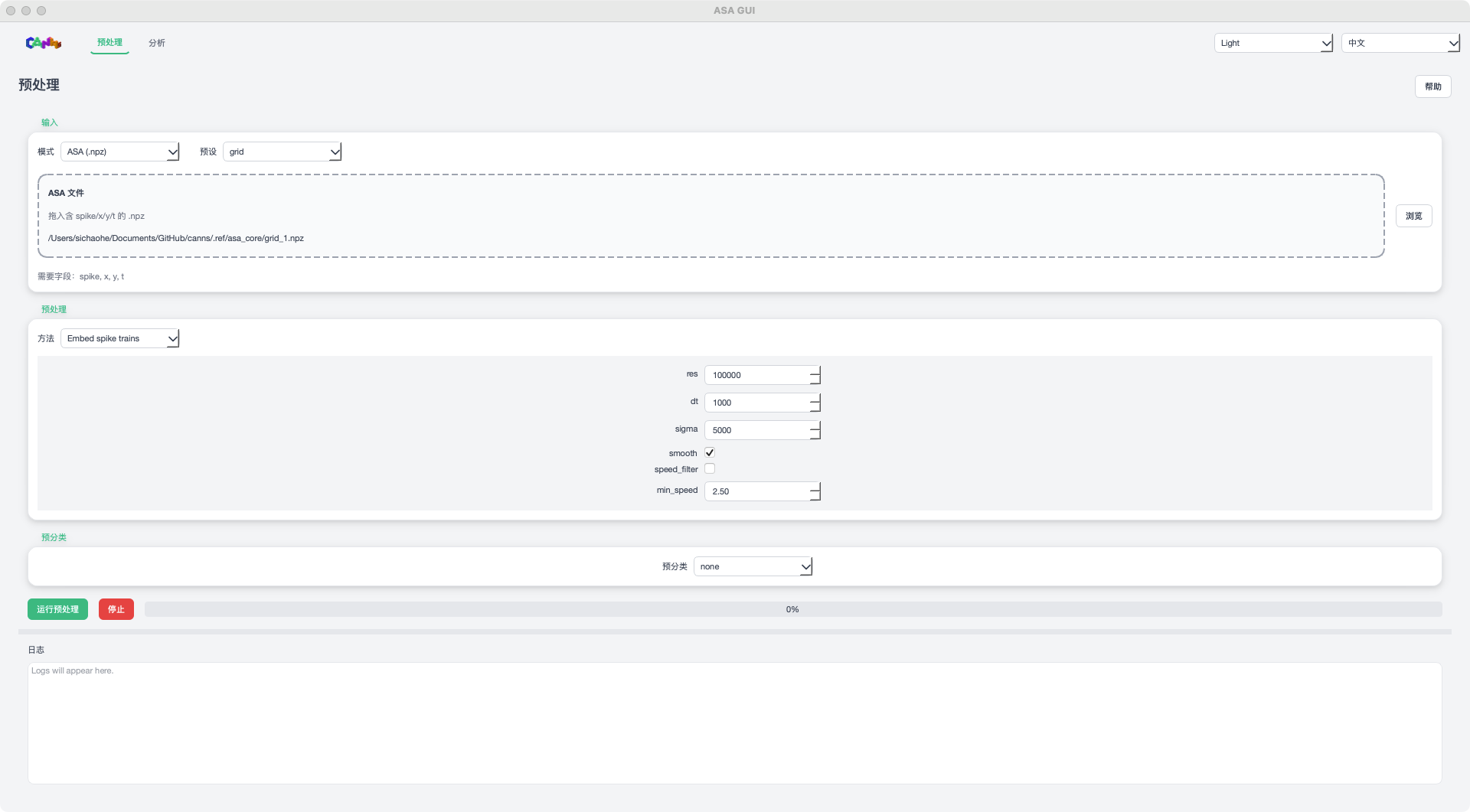
ASA GUI Preprocess page (placeholder image)

Analysis Page

Analysis Parameters	Select analysis modules and set parameters.
Analysis module	Supports TDA / CohoMap / PathCompare / CohoSpace / FR / FRM / GridScore.
Preprocess (Standardization)	StandardScaler standardization option.
Help	Opens quick help and common tips.
Language	Toggle interface language between Chinese and English.
Run Analysis / Stop / Progress	Run analysis and show progress.
Result Tabs	Barcode / CohoMap / Path Compare / CohoSpace / FR / FRM / GridScore / Files.
Files	Lists output files and allows Open Folder to open the results directory.

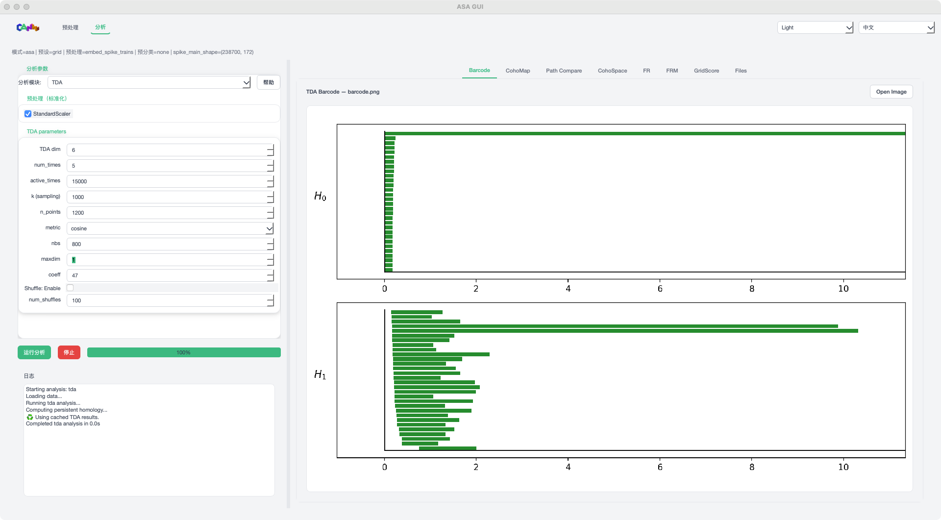
TDA mode example

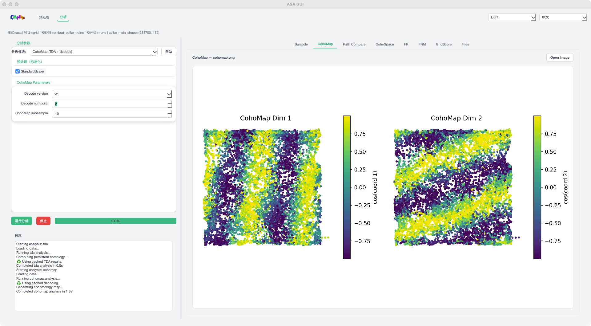
CohoMap mode example

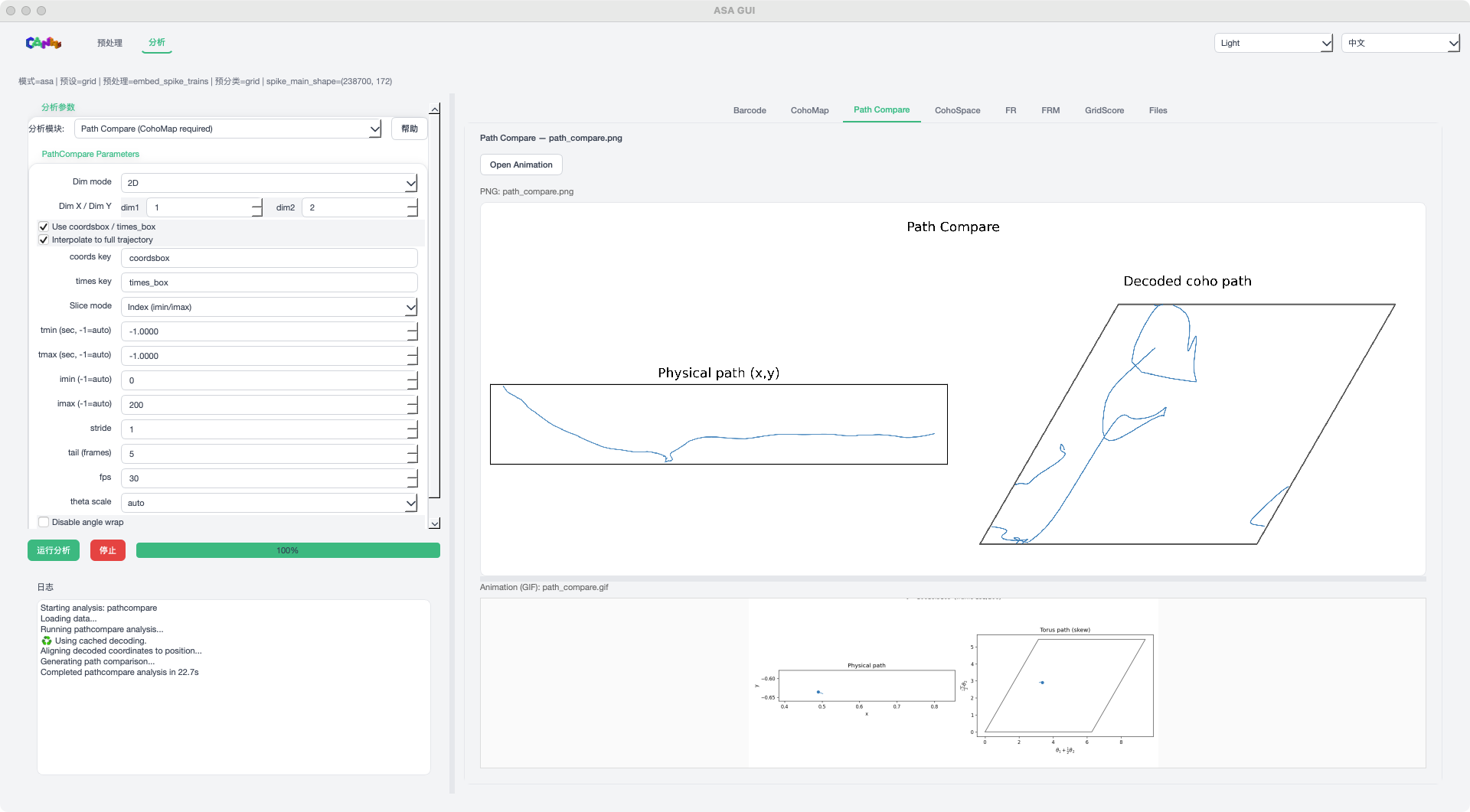
Path Compare mode example

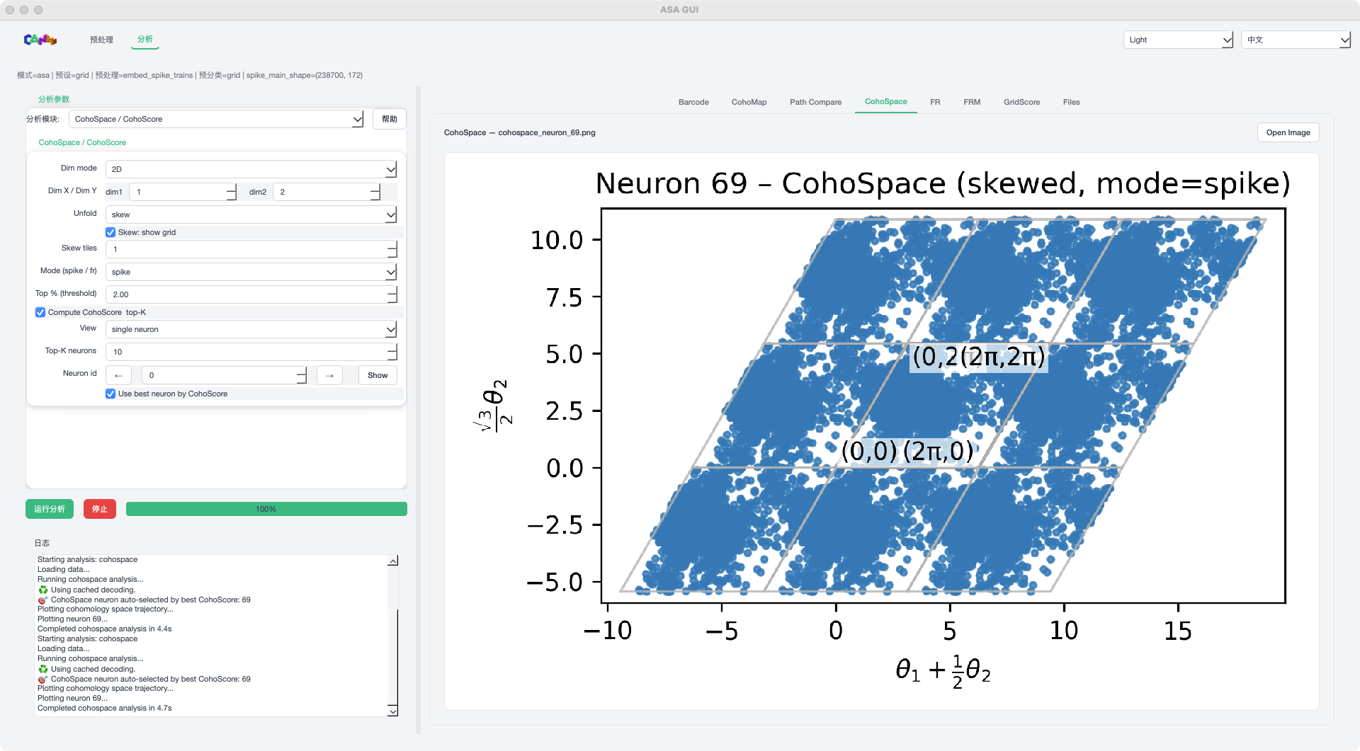
CohoSpace mode example

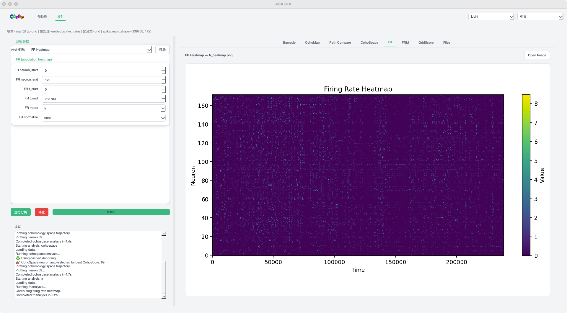
FR mode example

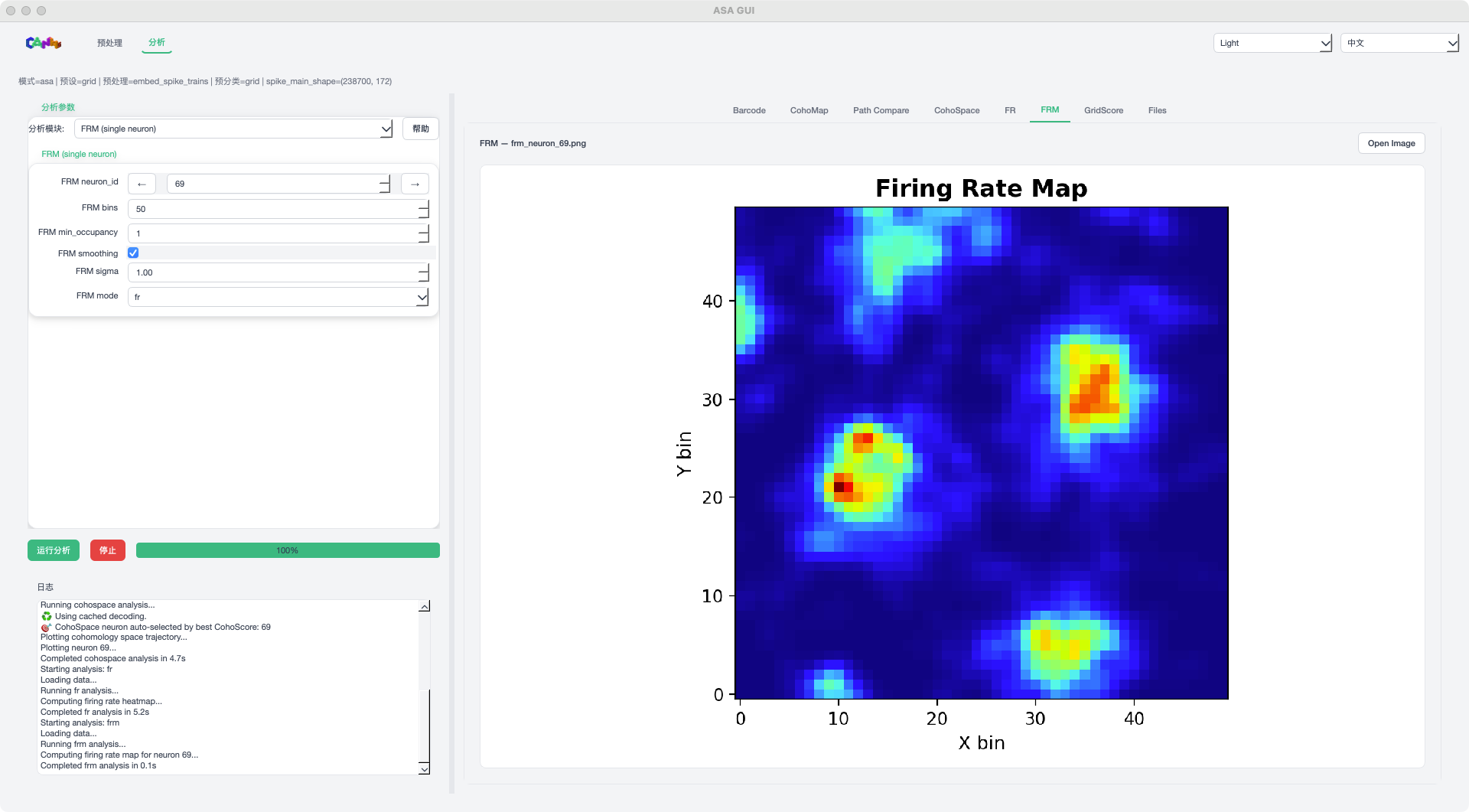
FRM mode example

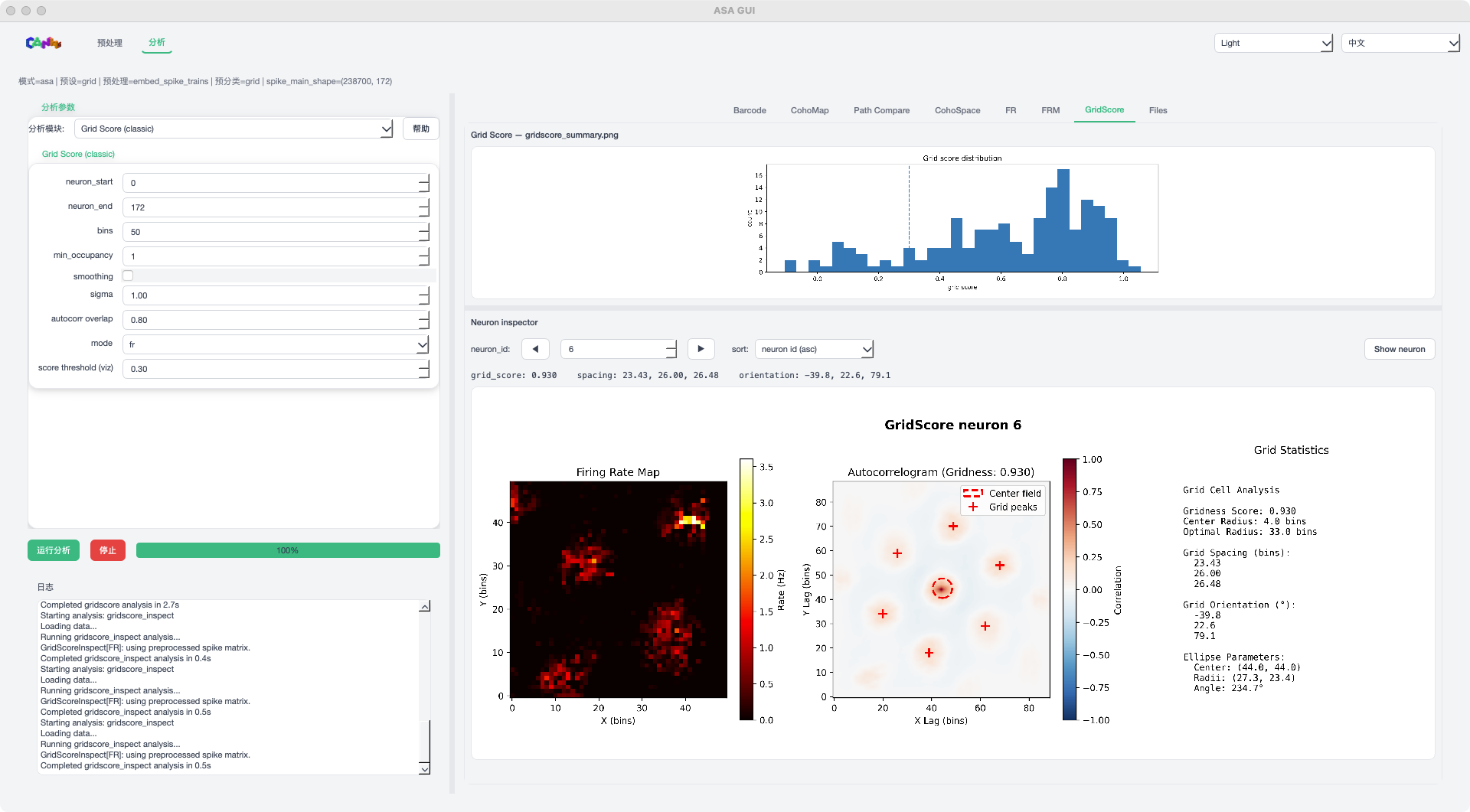
GridScore mode example

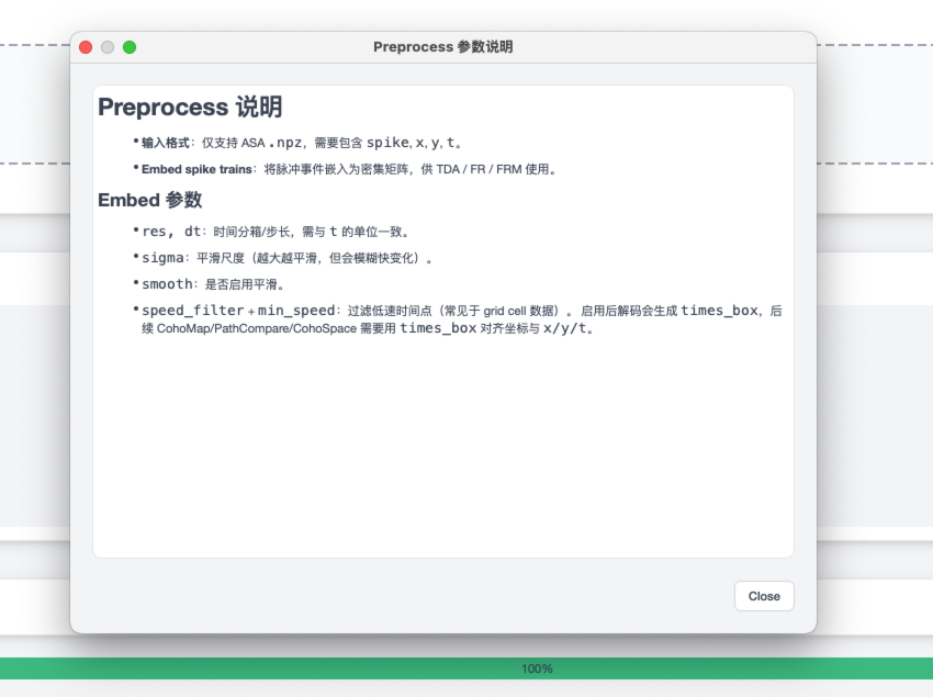
Preprocess help panel

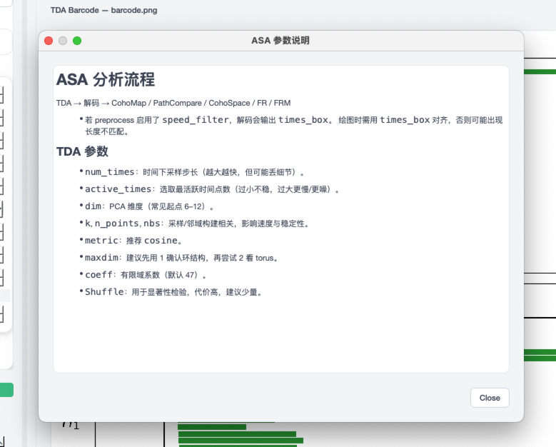
TDA help panel

Workflow Overview

1. Launch the ASA GUI

2. Select an ASA .npz input file

3. Configure preprocessing parameters and run Preprocess

4. Switch to the Analysis page and select an analysis module

5. Run the analysis and view results in the tabs

Step 1: Select ASA File

In the ASA file section, drag and drop or click Browse to select a .npz file. The interface will prompt for expected fields: spike / x / y / t.

ASA File Format

Must include at least spike and t:

• spike: A dense matrix of shape T x N, or a spike data structure suitable for embedding

• t: Time series (synchronized with spike)

• Optional: x / y for trajectory-related analyses

import numpy as np
np.savez(
    "session_asa.npz",
    spike=spike,
    t=t,
    x=x,
    y=y,
)

Step 2: Set Preprocessing

In the Preprocess section, choose a preprocessing method:

• None: Use the original spike structure directly

• Embed spike trains: Generate a dense matrix for use in TDA/FR/FRM

If embedding is required, set parameters such as res / dt / sigma / smooth / speed_filter / min_speed, then click Run Preprocess.

Step 3: Select Analysis Module

Switch to the Analysis page, choose an analysis module, and configure its parameters:

• TDA: Persistent homology analysis and barcode visualization

• CohoMap / CohoSpace: Decode and plot spatial structures

• Path Compare: Trajectory comparison (with animation output)

• FR / FRM: Firing rate heatmaps and neuron firing rate maps

• GridScore: Grid score computation and neuron browser

Click Run Analysis to start.

Step 4: View Results

After completion, view results in the right-hand tabs:

• Image Tabs: Support embedded preview and Open Image to open externally

• GridScore: Includes distribution plots and a neuron inspector

• Files: Lists output files and allows opening the output directory

Output Directory Structure

The output directory defaults to the current working directory:

Results/<dataset>_<hash>/

where <dataset> is derived from the input filename and <hash> is a prefix of the input hash. The directory contains analysis results and a cache (.asa_cache) to accelerate repeated runs.

Notes

• The GUI’s working directory is the current directory at launch time. Change directories in the terminal before launching if needed.

• For Neuron + Trajectory input, please use the ASA TUI or script-based workflow instead.