Tutorial 1: ASA Pipeline: End-to-End Decoding of Experimental Data

Objective: Learn how to run the ASA pipeline for experimental data using canns.analyzer.data, including TDA, phase decoding, CohoMap/CohoSpace, PathCompare, and FR/FRM.

Structure:

1. Data format and preparation

2. Embedding spike trains

3. TDA + Decoding

4. Cohomology Decoding + CohoMap / PathCompare

5. CohoSpace / CohoScore

6. FR Heatmap / FRM

Note

This tutorial demonstrates only Python-level API usage. For interactive operation, launch the GUI via python -m canns.pipeline.asa_gui or canns-gui (covered in detail in later sections).

.. note:: For background on topological decoding and population manifolds, see :cite:p:`Vaupel2023Duality,Gardner2022Toroidal`.

0. What ASA Can Do

ASA (Attractor Structure Analyzer) is designed for experimental scientists, linking population neural activity (spike / firing rate) with behavioral trajectories (x, y, t) into a reproducible analytical pipeline to discover and interpret hidden low-dimensional structures (e.g., ring / torus attractor manifolds).

Common scientific questions:

• Does the population activity exhibit topological structures such as rings / tori? (TDA)

• If such structures exist: how does the phase coordinate map onto the actual trajectory? (CohoMap)

• Does the decoded trajectory align with the true path? (PathCompare)

• Which neurons are most “concentrated/selective”? (CohoScore + CohoSpace)

• How can one quickly visualize population activity and single-unit raster plots? (FR / FRM)

The core ASA workflow relies on TDA and cocycle decoding, although FR/FRM can be used independently:

Input (ASA .npz: spike, x, y, t)
   → embed_spike_trains (optional)
   → TDA (persistent homology + cocycles)
   → Decode v2 (coords / coordsbox / times_box)
   → CohoMap / PathCompare / CohoSpace / CohoScore
   → FR / FRM

1. Data Format and Preparation

The ASA input is in .npz format and must contain at least:

• spike: neural activity (list-of-arrays / dict / (T, N))

• x, y: trajectory coordinates ((T,))

• t: timestamps ((T,))

This tutorial uses the built-in load_grid_data for demonstration. You can also replace it with your own experimental data.

from canns.data.loaders import load_grid_data

grid_data = load_grid_data()

print(f"Keys: {list(grid_data.keys())}")
print(f"t: {grid_data['t'].shape}, x: {grid_data['x'].shape}, y: {grid_data['y'].shape}")
print(f"spike type: {type(grid_data['spike'])}")

Loaded grid_1: 172 neurons
Position data available: 238700 time points
Keys: ['spike', 't', 'x', 'y']
t: (238700,), x: (238700,), y: (238700,)
spike type: <class 'numpy.ndarray'>

2. Embedding spike trains

When spike is a list-of-arrays / dict, it needs to be converted into a (T, N) dense matrix using embed_spike_trains.

from canns.analyzer import data

spike_cfg = data.SpikeEmbeddingConfig(
    smooth=True,
    speed_filter=False,
    min_speed=2.5,
)
spikes, xx, yy, tt = data.embed_spike_trains(grid_data, config=spike_cfg)

print(f"Embedded spikes: {spikes.shape}")

Embedded spikes: (238700, 172)

3. TDA + Decoding

Use tda_vis to obtain the persistent homology results, then decode the phase trajectories using decode_circular_coordinates_multi.

3.1 TDA Principle: From Point Cloud to Topology

In ASA, the population activity vector at each time point, A[t, :], is treated as a point in N-dimensional space. Thus, the T time points form a point cloud.

Intuition: If the network possesses an attractor/manifold (e.g., a bump moving along a ring), these points will cluster near a low-dimensional structure (ring / torus) rather than filling the entire N-dimensional space.

.. note:: For topology decoding related to ASA, see :cite:p:`Vaupel2023Duality` and :cite:p:`Gardner2022Toroidal`.

3.2 TDA Five-Step Pipeline in ASA

1. Temporal downsampling (num_times)

2. Select most active time points (active_times)

3. PCA dimensionality reduction (dim)

4. Point cloud denoising / representative sampling (k, n_points, metric)

5. Compute Persistent Homology (maxdim, coeff)

Practical recommendations:

• active_times is typically set to 5%–20% of the number of time points after downsampling

• First use maxdim=1 to detect loop structures, then consider maxdim=2 to examine torus-like features

3.3 From Cocycle to Angle: Why Phase Can Be Decoded

ripser returns cocycles (cohomology representatives) in PH computation. The ASA decoding process can be understood as follows:

• The cocycle provides structural information about “phase accumulation over one loop around the ring.”

• A phase function f is reconstructed via least squares (then mapped to θ = 2π f).

• The population activity is used to weight and obtain θ(t) over the full time series.

Important Note: The decoded θ represents the attractor phase and is not equivalent to the true x/y coordinates. Its actual physical interpretation requires visualization of how it unfolds along the trajectory via CohoMap.

3.4 The Role of Shuffle (Significance Testing)

When you suspect that the observed structure may arise from noise or sampling artifacts, you can enable shuffle:

• Repeat TDA on surrogate data that destroys topological structure while preserving certain statistical properties

• If the true barcode is significantly longer than the upper bound from shuffling, the structure is more credible

Note

Shuffling is computationally expensive; it is recommended to first run the main TDA and then perform a small number of shuffles as a sanity check.

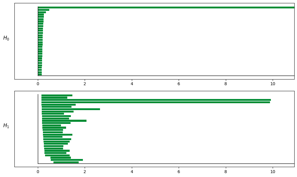
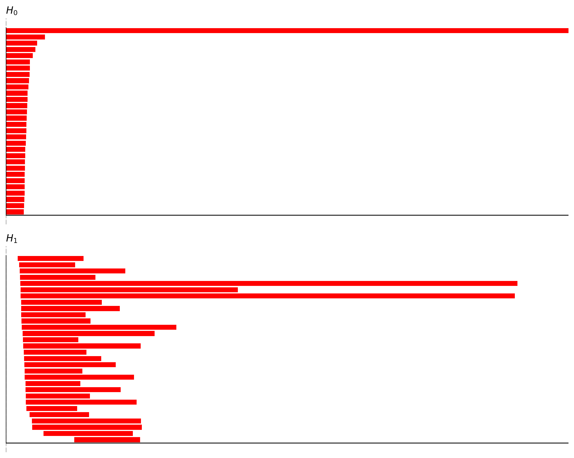
3.5 How to Read a Barcode (When to Use Shuffle)

In TDA/barcode.png, the key is to identify “significantly long bars”.

• H0 (connected components): Should eventually converge to 1 main branch (Betti0≈1)

• H1 (1-dimensional holes/loops): A ring typically shows 1 prominent long bar (Betti1≈1)

• H2 (2-dimensional voids): A torus typically shows 1 prominent long bar (Betti2≈1)

Why the torus often has (H0, H1, H2) ≈ (1, 2, 1):

• H1=2: There are two independent loop directions (can be thought of as “meridional/longitudinal”)

• H2=1: There is one 2-dimensional “shell” enclosing a void

Important

If you suspect a torus, set maxdim to 2 to observe H2. Otherwise, only H1 will be visible, which may lead to misclassifying it as a simple ring.

Empirical judgment and workflow:

• Round 1: Run the main TDA (without shuffle) first. If H1/H2 signals are strong, proceed directly to decode + CohoMap.

• Round 2 (optional): Perform a small number of shuffles as a sanity check only when the structure is unclear or noise is significant.

Note

Shuffle is not a default step: it serves more as a verification tool that should be enabled “only when in doubt”.

3.6 TDA Parameter Guide

Preprocess / embed:

• res, dt: Temporal binning; units must be consistent with t

• sigma: Smoothing scale (larger values yield smoother results but blur rapid changes)

• speed_filter, min_speed: Commonly used for grid cells; when enabled, rely on times_box for alignment

Core TDA parameters:

• num_times: Temporal downsampling step (larger values are faster but may lose details)

• active_times: Number of most active time points to select (too small leads to instability; too large increases computation time and noise)

• dim: PCA dimensionality (typical starting range: 6–12)

• k, n_points, nbs: Parameters for denoising, sampling, and distance graph construction (affect speed and stability)

• metric: cosine is recommended (insensitive to magnitude)

• maxdim: Start with 1; try 2 only after confirming the structure

• coeff: Coefficient for finite field (ASA default: 47)

Shuffle:

• Run the main TDA pipeline first, then perform a small number of shuffles

• Large-scale shuffling by default is not recommended (computationally expensive)

from canns.analyzer.visualization import PlotConfigs

# TDA
TDA_cfg = data.TDAConfig(maxdim=1, do_shuffle=False, show=True, progress_bar=True)
persistence = data.tda_vis(embed_data=spikes, config=TDA_cfg)

# Decode
grid_data_embedded = dict(grid_data)
grid_data_embedded["spike"] = spikes

decoding = data.decode_circular_coordinates_multi(
    persistence_result=persistence,
    spike_data=grid_data_embedded,
    num_circ=2,
)

print(decoding.keys())

Computing persistent homology for real data...

Completed H1 computation: 100%|██████████| 718201/718201 [00:05<00:00, 134504.22columns/s]

dict_keys(['coords', 'coordsbox', 'times', 'times_box', 'centcosall', 'centsinall'])

Decoded Output Key Fields

• coords: Decoded phases (T' × K)

• coordsbox: Phases used for alignment (T' × K)

• times_box: Alignment indices (T')

4. Cohomology Decoding: From Cocycle to Phase

Many people get stuck on “why can we decode the angle θ(t)?” ASA’s approach is as follows:

1. ripser returns a cocycle (a cohomology representative)

2. Select a threshold close to death (commonly birth + 0.99*(death-birth))

3. Solve a least-squares problem to recover “phases at points” from “phase differences on edges”

4. Map f ∈ [0,1) to θ = 2π f

5. Extend to all time points using population activity weighting to obtain θ(t)

Intuitive summary:

• The cocycle provides a reference frame in which “the phase accumulates by one full cycle when looping around a hole”

• Population activity extends this reference frame to all time points

4.1 Phase and Physical Space: Key Points

• θ(t) is the attractor phase, not a direct substitute for x/y

• In the torus scenario, θ1/θ2 are more like “folded periodic phases”

• Correct interpretation: use CohoMap to project the phase back onto the real trajectory and observe the unwrapping behavior

Alignment considerations:

• Use times_box to align decoding results with x/y/t

• The difference between coords and coordsbox handles speed filtering and sampling alignment

Alignment example (using times_box):

t_use, x_use, y_use, coords_use, _ = data.align_coords_to_position_2d(
    t_full=np.asarray(grid_data["t"]).ravel(),
    x_full=np.asarray(grid_data["x"]).ravel(),
    y_full=np.asarray(grid_data["y"]).ravel(),
    coords2=np.asarray(decoding["coords"]),
    use_box=True,
    times_box=decoding.get("times_box", None),
    interp_to_full=True,
)

coords_use = data.apply_angle_scale(coords_use, "rad")

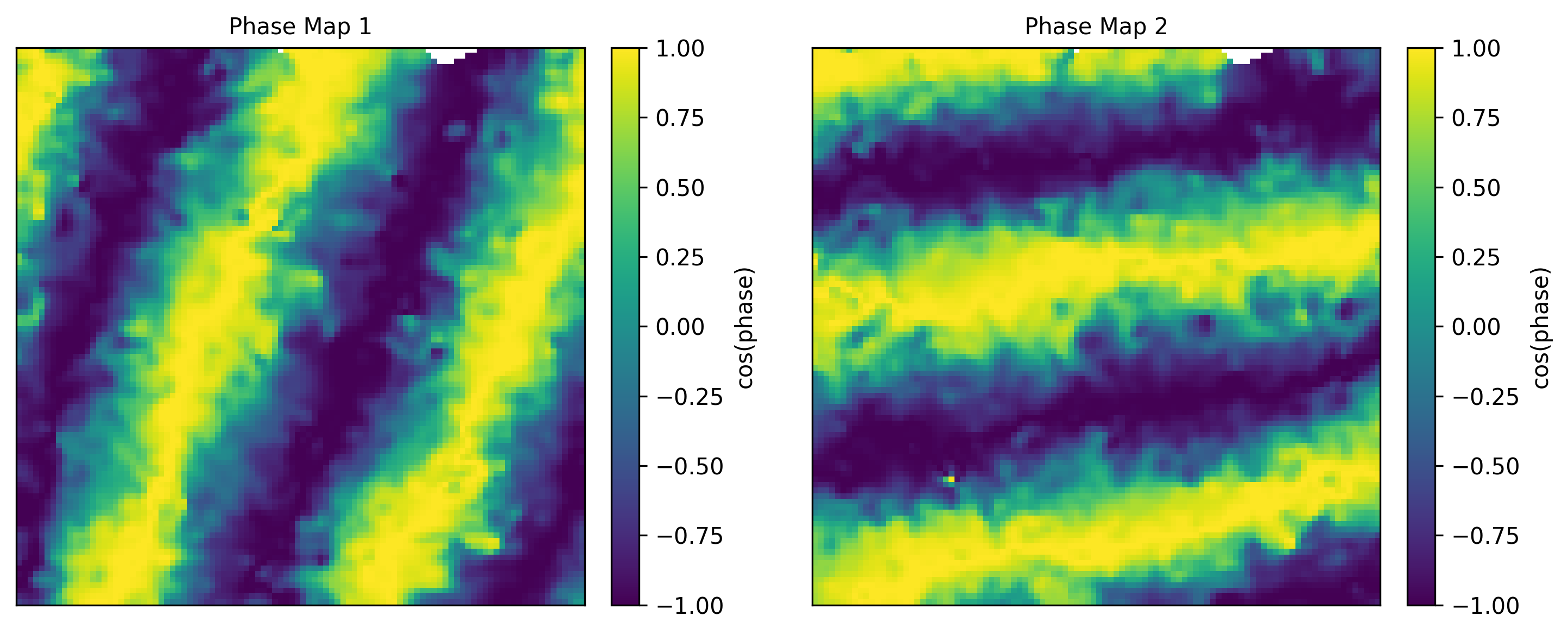
4.2 CohoMap and PathCompare

• plot_cohomap_multi projects phase trajectories onto real trajectories

• plot_path_compare_1d / plot_path_compare_2d align real paths with decoded paths

.. note:: Refer to the corresponding example scripts: ``examples/experimental_data_analysis/path_compare1d.py`` and ``examples/experimental_data_analysis/path_compare2d.py``.

import numpy as np
from canns.analyzer.visualization import PlotConfigs

# CohoMap
cohomap_cfg = PlotConfigs.cohomap(show=True)

data.plot_cohomap_multi(
    decoding_result=decoding,
    position_data={"x": grid_data["x"], "y": grid_data["y"]},
    config=cohomap_cfg,
)

# PathCompare
coords = np.asarray(decoding.get("coords"))

t_use, x_use, y_use, coords_use, _ = data.align_coords_to_position_2d(
    t_full=np.asarray(grid_data["t"]).ravel()[200:260],
    x_full=np.asarray(grid_data["x"]).ravel()[200:260],
    y_full=np.asarray(grid_data["y"]).ravel()[200:260],
    coords2=coords,
    use_box=True,
    times_box=decoding.get("times_box", None),
    interp_to_full=True,
)

coords_use = data.apply_angle_scale(coords_use, "rad")

path_cfg = PlotConfigs.path_compare_2d(show=True)

data.plot_path_compare_2d(x_use, y_use, coords_use, config=path_cfg)

(<Figure size 1200x500 with 2 Axes>,
 array([<Axes: title={'center': 'Physical path (x,y)'}>,
        <Axes: title={'center': 'Decoded coho path'}>], dtype=object))

5. CohoSpace / CohoScore

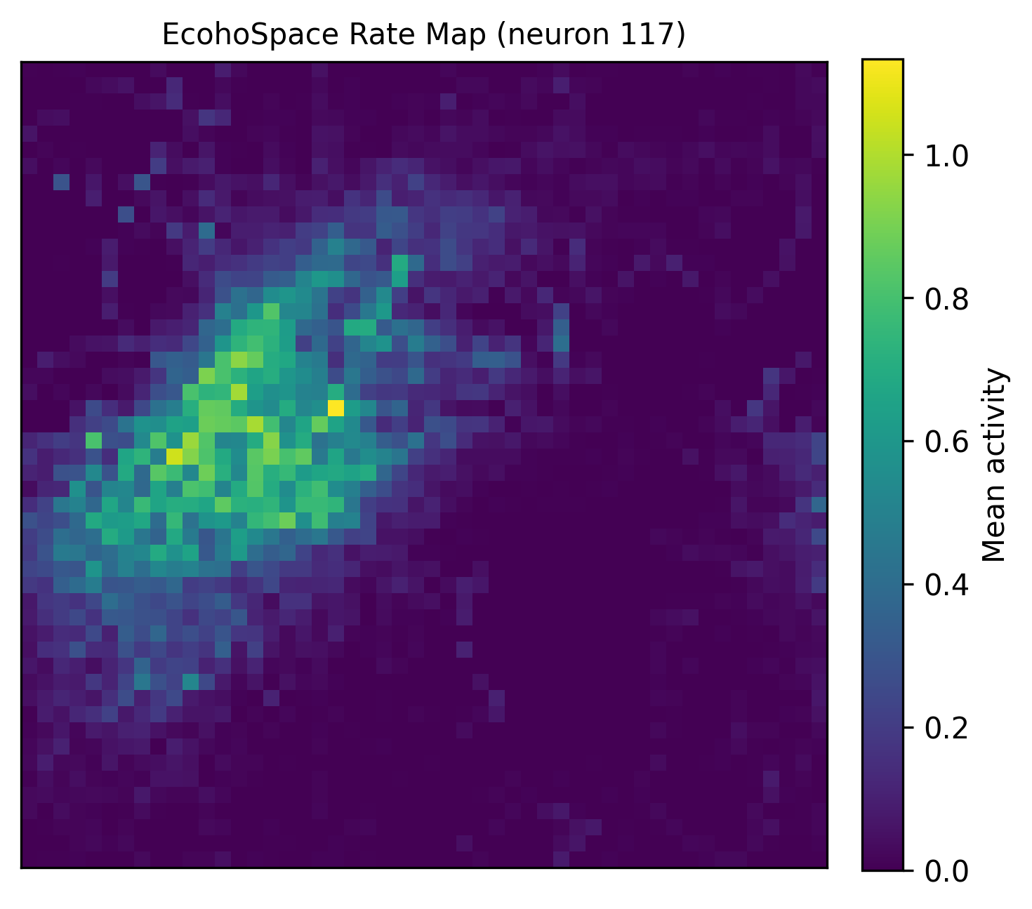
CohoSpace is used to visualize the preference distribution of neurons in phase space.

.. note:: For the corresponding example scripts, please refer to: ``examples/experimental_data_analysis/cohospace1d.py`` and ``examples/experimental_data_analysis/cohospace2d.py``.

coords = np.asarray(decoding.get("coords"))
coordsbox = np.asarray(decoding.get("coordsbox"))

traj_cfg = PlotConfigs.cohospace_trajectory_2d(show=True)

data.plot_cohospace_trajectory_2d(
    coords=coords[:, :2],
    times=None,
    subsample=2,
    config=traj_cfg,
)

neuron_cfg = PlotConfigs.cohospace_neuron_2d(show=True)

fig = data.plot_cohospace_neuron_2d(
    coords=coordsbox[:, :2],
    activity=spikes,
    neuron_id=130,
    mode="fr",
    top_percent=1,
    config=neuron_cfg,
)

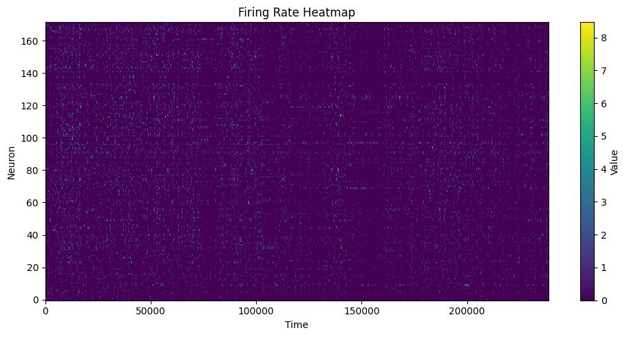
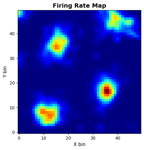
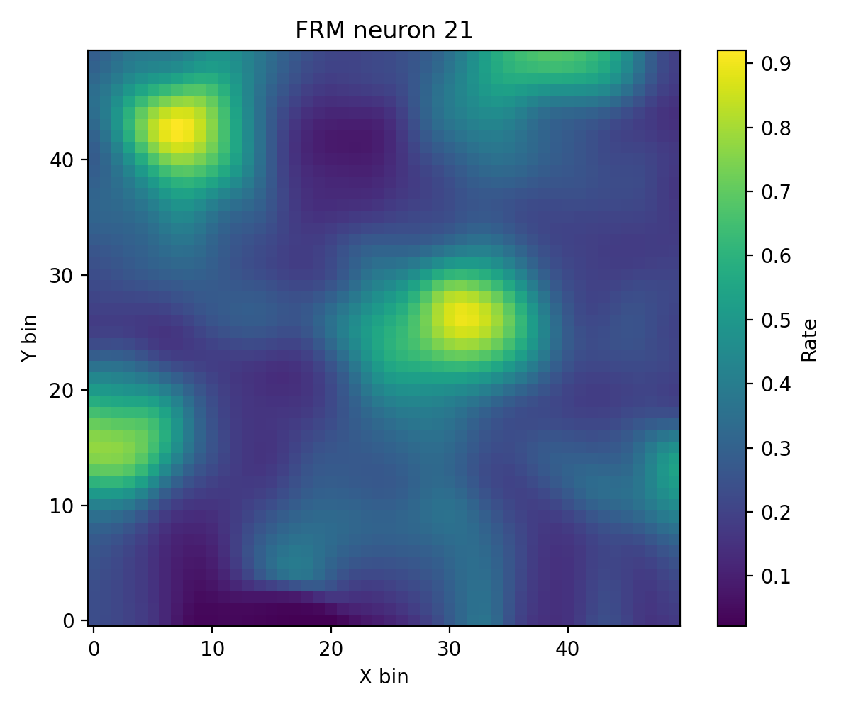
6. FR Heatmap / FRM

• compute_fr_heatmap_matrix: Population firing rate heatmap

• compute_frm: Single-neuron spatial firing map

# FR Heatmap
heatmap = data.compute_fr_heatmap_matrix(spikes, transpose=True)
heatmap_cfg = PlotConfigs.fr_heatmap(show=True)

data.save_fr_heatmap_png(heatmap, config=heatmap_cfg)

# FRM
frm_res = data.compute_frm(
    spikes,
    grid_data["x"],
    grid_data["y"],
    neuron_id=130,
    bins=50,
    min_occupancy=1,
    smoothing=True,
    sigma=1.0,
    nan_for_empty=True,
)

frm_cfg = PlotConfigs.frm(show=True)

data.plot_frm(frm_res.frm, config=frm_cfg, dpi=200)

Visual Examples

TDA barcode	CohoMap phase projection
CohoSpace neuron preference	Single-neuron FRM

Related example scripts

• examples/experimental_data_analysis/tda_vis.py

• examples/experimental_data_analysis/cohomap.py

• examples/experimental_data_analysis/cohospace1d.py

• examples/experimental_data_analysis/cohospace2d.py

• examples/experimental_data_analysis/path_compare1d.py

• examples/experimental_data_analysis/path_compare2d.py

• examples/experimental_data_analysis/firing_rate_heatmap.py

• examples/experimental_data_analysis/firing_field_map.py

• examples/cell_classification