Design Philosophy

This notebook captures the design philosophy of the Continuous Attractor Neural Networks (CANNs) Python library so newcomers can understand each module quickly.

The library centres on CANNs and offers a unified high-level API for loading, analysing, and training state-of-the-art architectures, enabling researchers and developers to iterate on brain-inspired workflows efficiently.

Module Overview

• model Built-in model package.

  • basic Core CANN models and their variants.

  • brain_inspired Brain-inspired models.

  • hybrid Hybrid models mixing CANNs with ANNs or other mechanisms.

• task Task utilities for CANNs, covering generation, persistence, import, and visualisation.

• analyzer Analysis helpers focused on visualisation.

  • model analyzer Tools for examining CANN models, including energy landscapes, firing rates, and tuning curves.

  • data analyzer Routines for experimental-data-driven CANN analysis or dynamical inspection of virtual RNN models.

• trainer Unified training and prediction interfaces.

• pipeline End-to-end flows that combine the above packages for streamlined execution.

Module Walkthrough

models

Overview

The models package implements base CANNs across different dimensionalities, brain-inspired variants, and hybrid combinations. It underpins the rest of the library and inter-operates with other modules to support varied scenarios.

The implementations are grouped by type:

• Basic Models (canns.models.basic) Canonical CANN architectures and their variants.

• Brain-Inspired Models (canns.models.brain_inspired) Brain-inspired network implementations.

• Hybrid Models (canns.models.hybird) Hybrids that couple CANNs with ANNs or other mechanisms.

These models rely on the Brain Simulation Ecosystem, especially brainstate. brainstate—backed by JAX/BrainUnit—provides the brainstate.nn.Dynamics abstraction, State/HiddenState/ParamState containers, unified time-step control via brainstate.environ, and utilities such as brainstate.compile.for_loop and brainstate.random. With these building blocks, CANN implementations only describe variables and update rules while brainstate handles time stepping, parallelism, and randomness, lowering implementation overhead.

Usage Examples

The following examples summarise the end-to-end workflow, see examples/cann/cann1d_oscillatory_tracking.py, examples/cann/cann2d_tracking.py, and examples/brain_inspired/hopfield_train.py.

import brainstate as bst
from canns.models.basic import CANN1D, CANN2D
from canns.task.tracking import SmoothTracking1D, SmoothTracking2D
from canns.analyzer.plotting import (
    PlotConfigs,
    energy_landscape_1d_animation,
    energy_landscape_2d_animation,
)

bst.environ.set(dt=0.1)

# Create a 1D CANN instance and initialise its state
cann = CANN1D(num=512)  # 512 neurons
cann.init_state()       # Initialise the neural network state

# Use a SmoothTracking1D task (described later) to generate stimuli
task_1d = SmoothTracking1D(
    cann_instance=cann,
    Iext=(1.0, 0.75, 2.0, 1.75, 3.0),
    duration=(10.0,) * 4,
    time_step=bst.environ.get_dt(),
)
task_1d.get_data()  # Generate task data

# Define a step function that applies the stimulus to the CANN
def step_1d(_, stimulus):
    cann(stimulus)                          # Update the CANN state with the provided stimulus
    return cann.u.value, cann.inp.value     # Return membrane potential and external input

us, inputs = bst.compile.for_loop(step_1d, task_1d.run_steps, task_1d.data) # Run the step function via brainstate.compile.for_loop

<SmoothTracking1D> Generating Task data: 400it [00:00, 2409.20it/s]

For brain-inspired models, refer to the Hopfield example (examples/brain_inspired/hopfield_train.py) to perform pattern recovery from noisy images.

from canns.models.brain_inspired import AmariHopfieldNetwork
from canns.trainer import HebbianTrainer

# Instantiate the Amari Hopfield network and initialise its state
model = AmariHopfieldNetwork(num_neurons=128 * 128, asyn=False, activation='sign')
model.init_state()  # Initialise the neural network state

trainer = HebbianTrainer(model) # Create the HebbianTrainer (explained later in this notebook)
trainer.train(train_patterns)  # `train_patterns`: List[np.ndarray] of shape (N,) used for training
denoised = trainer.predict_batch(noisy_patterns, show_sample_progress=True)

Extension Guidelines

Because the core implementations depend on brainstate, consult the official documentation (https://brainstate.readthedocs.io) when extending models. Key topics include registering states with nn.Dynamics, managing time via environ.set/get_dt, batching updates with compile.for_loop, and working with ParamState/HiddenState. Mastering these concepts helps produce numerics and APIs that interoperate with existing components.

For basic models

Each model inherits from canns.models.basic.BasicModel or BasicModelGroup. Typical tasks include:

• Call the parent constructor in __init__ (e.g. super().__init__(math.prod(shape), **kwargs)) and store shape, varshape, or related dimensions.

• Implement make_conn() to build the connectivity matrix and assign it to self.conn_mat (see the Gaussian kernel implementation in src/canns/models/basic/cann.py).

• Implement get_stimulus_by_pos(pos) so tasks can request external stimuli from feature-space positions.

• Register brainstate.HiddenState/State objects in init_state() (commonly self.u, self.r, self.inp) to ensure updates can read and write directly.

• Write the single-step dynamics inside update(inputs) and scale by brainstate.environ.get_dt() for numerical stability.

• Expose diagnostic values or axes (such as self.x or self.rho) through properties for reuse by tasks, analyzers, and pipelines.

For brain-inspired models

Models inherit from canns.models.brain_inspired.BrainInspiredModel or BrainInspiredModelGroup. To extend them:

• Register the state vector (default self.s) and weight matrix self.W inside init_state(); store weights in a brainstate.ParamState so Hebbian learning can write back directly.

• Override weight_attr if the weight field is not called W, allowing HebbianTrainer to locate it.

• Implement update(...) and the energy property so the trainer can run the generic prediction loop and detect convergence.

• Implement apply_hebbian_learning(patterns) when customised Hebbian rules are required; otherwise rely on the trainer’s generic update.

• Override resize(num_neurons, preserve_submatrix=True) if the model supports dynamic resizing (see src/canns/models/brain_inspired/hopfield.py).

For hybrid models

Future work (待补充 / TBD).

task

Overview

The task package generates, saves, loads, imports, and visualises CANN-specific stimuli. It offers predefined task types while allowing custom extensions for specialised needs.

Usage Examples

For a one-dimensional tracking task (see examples/cann/cann1d_oscillatory_tracking.py):

from canns.task.tracking import SmoothTracking1D
from canns.models.basic import CANN1D
from canns.analyzer.plotting import energy_landscape_1d_animation, PlotConfigs

# Create a SmoothTracking1D task
task_st = SmoothTracking1D(
    cann_instance=cann,
    Iext=(1., 0.75, 2., 1.75, 3.),   # External input amplitudes for each phase of the SmoothTracking1D task
    duration=(10., 10., 10., 10.),   # Duration of each phase (four phases of 10 time units)
    time_step=bst.environ.get_dt(),
)
task_st.get_data()  # Generate task data

task_st.data  # Task data containing the time series and corresponding stimuli

<SmoothTracking1D> Generating Task data: 400it [00:00, 9206.62it/s]

array([[0.10189284, 0.09665093, 0.09165075, ..., 0.11314222, 0.10738649,
        0.10189275],
       [0.10079604, 0.09560461, 0.09065294, ..., 0.11193825, 0.10623717,
        0.10079593],
       [0.09970973, 0.0945684 , 0.08966482, ..., 0.11074577, 0.10509886,
        0.09970973],
       ...,
       [9.72546482, 9.68417931, 9.64015198, ..., 9.79967213, 9.76397419,
        9.72546482],
       [9.76497078, 9.72653675, 9.68532467, ..., 9.83337116, 9.80059338,
        9.76497078],
       [9.80151176, 9.76596642, 9.72760582, ..., 9.86403942, 9.8342123 ,
        9.80151081]], shape=(400, 512))

SmoothTracking1D and SmoothTracking2D automatically interpolate smooth trajectories from key points. task.data and task.Iext_sequence can be consumed directly by models or analyzers.

Every task inherits the base save_data/load_data helpers for repeatable experiments:

task.save_data("outputs/tracking_task.npz")
# ... later or on another machine
restored = SmoothTracking1D(
    cann_instance=cann_model,
    Iext=(1.0, 0.8, 2.2, 1.5),
    duration=(8.0,) * 3,
    time_step=bst.environ.get_dt(),
)
restored.load_data("outputs/tracking_task.npz")

Data successfully saved to: outputs/tracking_task.npz
Data successfully loaded from: outputs/tracking_task.npz

When self.data is a dataclass (for example OpenLoopNavigationData), the base class serialises individual fields and reconstructs the structured object on load.

OpenLoopNavigationTask can synthesise trajectories or import recordings. See examples/cann/theta_sweep_grid_cell_network.py for the analysis flow and examples/cann/import_external_trajectory.py for trajectory import.

import numpy as np
import os
from canns.task.open_loop_navigation import OpenLoopNavigationTask

# Load external position data with NumPy
data = np.load(os.path.join(os.getcwd(), "..", "..", "en", "notebooks", "external_trajectory.npz"))
positions = data["positions"]  # Shape: (time_steps, 2)
times = data["times"]          # Shape: (time_steps,)
simulate_time = times[-1] - times[0]
env_size = 1.8
dt = 0.1

task = OpenLoopNavigationTask(duration=simulate_time, width=env_size, height=env_size, dt=dt)
task.import_data(position_data=positions, times=times)  # Import the external position data
task.calculate_theta_sweep_data()   # Compute theta-sweep features
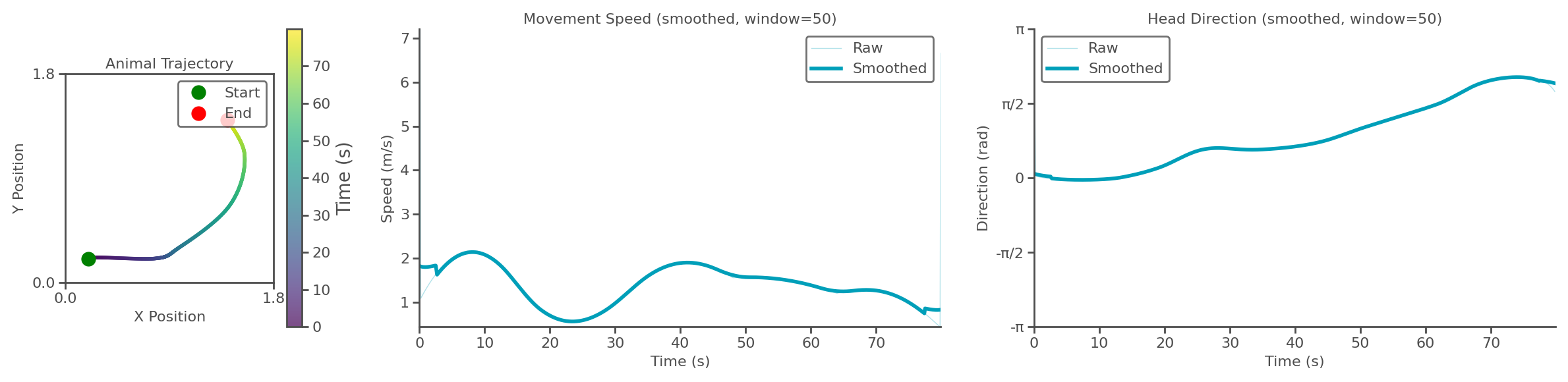
task.show_trajectory_analysis(save_path="trajectory.png", show=True, smooth_window=50) # Visualise the trajectory analysis

Successfully imported trajectory data with 800 time steps
Spatial dimensions: 2D
Time range: 0.000 to 1.598 s
Mean speed: 1.395 units/s
Trajectory analysis saved to: trajectory.png

Extension Guidelines

To build a custom task, inherit canns.task.Task and follow these steps:

• Parse configuration in the constructor and optionally set data_class.

• Implement get_data() to generate or load data, storing the output in self.data (either a numpy.ndarray or a dataclass).

• Provide import helpers such as import_data(...) when external data must match the self.data structure.

• Implement show_data(show=True, save_path=None) for the most relevant visualisation.

• Reuse the base save_data/load_data for persistence instead of re-implementing them.

analyzer

Overview

The analyzer package supplies tools for inspecting CANN models and experimental datasets. It spans two categories: model analysis and data analysis.

Usage

Model analysis

After combining a model with a task, invoke analyzer helpers to produce visualisations. Continuing the 1D tracking workflow:

import brainstate
from canns.task.tracking import SmoothTracking1D
from canns.models.basic import CANN1D
from canns.analyzer.plotting import energy_landscape_1d_animation, PlotConfigs

brainstate.environ.set(dt=0.1)



# Create a SmoothTracking1D task
task_st = SmoothTracking1D(
    cann_instance=cann,
    Iext=(1., 0.75, 2., 1.75, 3.),   # External input amplitudes for each phase of the SmoothTracking1D task
    duration=(10., 10., 10., 10.),   # Duration of each phase (four phases of 10 time units)
    time_step=brainstate.environ.get_dt(),
)
task_st.get_data()  # Generate task data


# Define a step function that drives the CANN with the generated inputs
def run_step(t, inputs):
    cann(inputs)
    return cann.u.value, cann.inp.value

# Execute the loop with brainstate.compile.for_loop
us, inps = brainstate.compile.for_loop(
    run_step,
    task_st.run_steps,  # Total number of simulation steps
    task_st.data,       # Task data produced by SmoothTracking1D
    pbar=brainstate.compile.ProgressBar(10) # Update the progress bar every 10 iterations
)

# Configure and generate the energy landscape animation
config = PlotConfigs.energy_landscape_1d_animation(
    time_steps_per_second=100,
    fps=20,
    title='Smooth Tracking 1D',
    xlabel='State',
    ylabel='Activity',
    repeat=True,
    save_path='smooth_tracking_1d.gif',
    show=False
)

# Render the energy landscape animation
energy_landscape_1d_animation(
    data_sets={'u': (cann.x, us), 'Iext': (cann.x, inps)},
    config=config
)

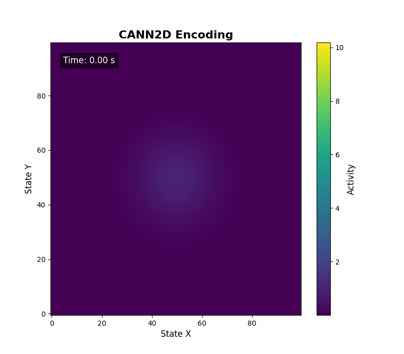
For two-dimensional activity, call energy_landscape_2d_animation(zs_data=...) to render the heat map.

Data analysis

Follow the repository scripts for end-to-end workflows:

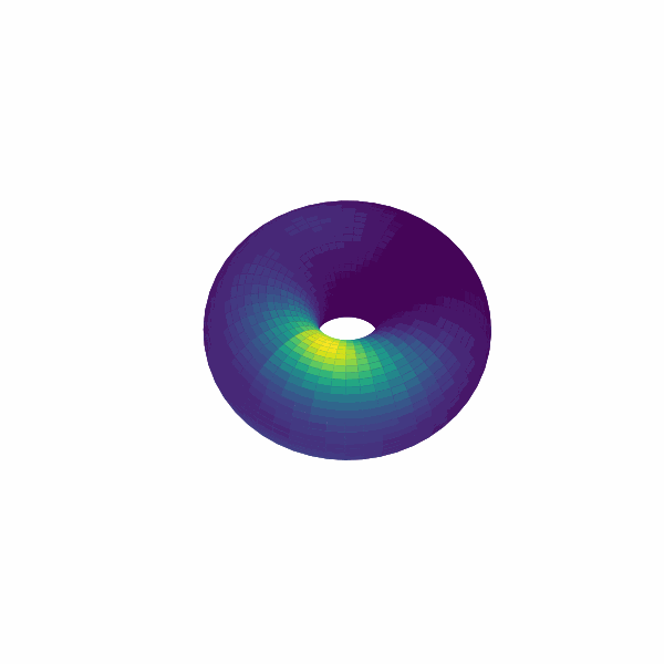
• examples/experimental_cann1d_analysis.py: load_roi_data() loads sample ROI traces, then bump_fits and create_1d_bump_animation fit and animate 1D bumps.

• examples/experimental_cann2d_analysis.py: after embed_spike_trains, use UMAP and plot_projection for dimensionality reduction, then call tda_vis, decode_circular_coordinates, and plot_3d_bump_on_torus for topological analysis and torus animation.

Extension Guidelines

Model analysis

Although analyzers share no base class, follow the preset pattern in src/canns/analyzer/plotting/config.py: parameterise titles, axes, frame rates, and other options through PlotConfig/PlotConfigs, and accept a config object in plotting functions. This keeps visual interfaces consistent and easy to customise.

Data analysis

Likewise, data-analysis helpers have no common base. Implement custom utilities as required for specific datasets.

trainer

Overview

The trainer package exposes unified interfaces for training and evaluating brain-inspired models. It currently focuses on Hebbian learning, with room to add additional strategies later.

Usage

Refer to examples/brain_inspired/hopfield_train.py for HebbianTrainer in practice:

import numpy as np
import skimage.data
from matplotlib import pyplot as plt
from skimage.color import rgb2gray
from skimage.filters import threshold_mean
from skimage.transform import resize

from canns.models.brain_inspired import AmariHopfieldNetwork
from canns.trainer import HebbianTrainer

np.random.seed(42)

def preprocess_image(img, w=128, h=128) -> np.ndarray:
    """Resize, grayscale (if needed), threshold to binary, then map to {-1,+1}."""
    if img.ndim == 3:
        img = rgb2gray(img)
    img = resize(img, (w, h), anti_aliasing=True)
    img = img.astype(np.float32, copy=False)
    thresh = threshold_mean(img)
    binary = img > thresh
    shift = np.where(binary, 1.0, -1.0).astype(np.float32)
    return shift.reshape(w * h)

# Load training images from skimage
camera = preprocess_image(skimage.data.camera())
astronaut = preprocess_image(skimage.data.astronaut())
horse = preprocess_image(skimage.data.horse().astype(np.float32))
coffee = preprocess_image(skimage.data.coffee())

data_list = [camera, astronaut, horse, coffee]

# Instantiate the Amari Hopfield network and initialise its state
model = AmariHopfieldNetwork(num_neurons=data_list[0].shape[0], asyn=False, activation="sign")
model.init_state()

# Create the HebbianTrainer and train the network
trainer = HebbianTrainer(model)
trainer.train(data_list)

# Create noisy test patterns
def get_corrupted_input(input, corruption_level):
    corrupted = np.copy(input)
    inv = np.random.binomial(n=1, p=corruption_level, size=len(input))
    for i, v in enumerate(input):
        if inv[i]:
            corrupted[i] = -1 * v
    return corrupted

tests = [get_corrupted_input(d, 0.3) for d in data_list]

# Predict the denoised patterns
predicted = trainer.predict_batch(tests, show_sample_progress=True)

# Visualise the predictions
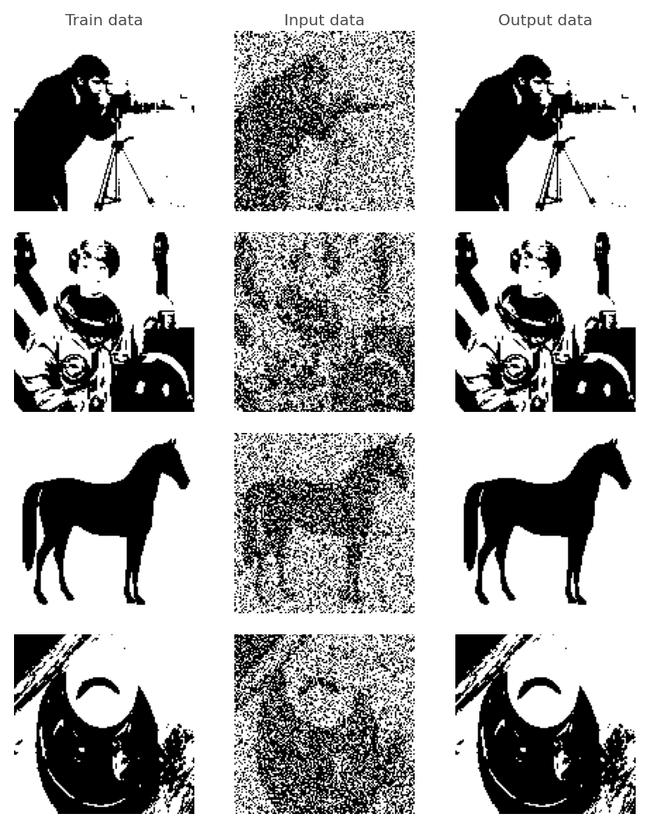
def plot(data, test, predicted, figsize=(5, 6)):
    def reshape(data):
        dim = int(np.sqrt(len(data)))
        data = np.reshape(data, (dim, dim))
        return data

    data = [reshape(d) for d in data]
    test = [reshape(d) for d in test]
    predicted = [reshape(d) for d in predicted]

    fig, axarr = plt.subplots(len(data), 3, figsize=figsize)
    for i in range(len(data)):
        if i==0:
            axarr[i, 0].set_title('Train data')
            axarr[i, 1].set_title("Input data")
            axarr[i, 2].set_title('Output data')

        axarr[i, 0].imshow(data[i], cmap='gray')
        axarr[i, 0].axis('off')
        axarr[i, 1].imshow(test[i], cmap='gray')
        axarr[i, 1].axis('off')
        axarr[i, 2].imshow(predicted[i], cmap='gray')
        axarr[i, 2].axis('off')

    plt.tight_layout()
    plt.savefig("discrete_hopfield_train.png")
    plt.show()


plot(data_list, tests, predicted, figsize=(5, 6))

Processing samples: 100%|█████████████| 4/4 [00:04<00:00,  1.05s/it, sample=4/4]

Extension Guidelines

To introduce a new trainer, inherit canns.trainer.Trainer and:

• Capture the target model and progress settings in the constructor.

• Implement train(self, train_data) to define the parameter update rule.

• Implement predict(self, pattern, *args, **kwargs) for single-sample inference, using predict_batch for batching when appropriate.

• Honour the default configure_progress contract so users can toggle iteration progress or compilation.

• Agree on shared attribute names (for example weights or state vectors) when the trainer cooperates with specific models.

Pipeline

Overview

The pipeline package chains models, tasks, analyzers, and trainers into end-to-end workflows so that common needs are satisfied with minimal user code.

Usage

Run ThetaSweepPipeline for a full workflow (see examples/pipeline/theta_sweep_from_external_data.py):

from canns.pipeline import ThetaSweepPipeline

pipeline = ThetaSweepPipeline(
    trajectory_data=positions,
    times=times,
    env_size=env_size,
)
results = pipeline.run(output_dir="theta_sweep_results")

🚀 Starting Theta Sweep Pipeline...
📊 Setting up spatial navigation task...
Successfully imported trajectory data with 800 time steps
Spatial dimensions: 2D
Time range: 0.000 to 1.598 s
Mean speed: 1.395 units/s
🧠 Setting up neural networks...
⚡ Running theta sweep simulation...

/Users/sichaohe/Documents/GitHub/canns/.venv/lib/python3.12/site-packages/tqdm/auto.py:21: TqdmWarning: IProgress not found. Please update jupyter and ipywidgets. See https://ipywidgets.readthedocs.io/en/stable/user_install.html
  from .autonotebook import tqdm as notebook_tqdm
Running for 800 iterations: 100%|██████████| 800/800 [00:10<00:00, 75.01it/s]

📈 Generating trajectory analysis...
Trajectory analysis saved to: theta_sweep_results/trajectory_analysis.png
📊 Generating population activity plot...
Plot saved to: theta_sweep_results/population_activity.png
🎬 Creating theta sweep animation...
[theta_sweep] Using imageio backend for theta sweep animation (auto-detected).
[theta_sweep] Detected JAX; using 'spawn' start method to avoid fork-related deadlocks.

<theta_sweep> Rendering frames: 100%|██████████| 80/80 [03:42<00:00,  2.78s/it]

✅ Pipeline completed successfully!
📁 Results saved to: /Users/sichaohe/Documents/GitHub/canns/docs/zh/notebooks/theta_sweep_results

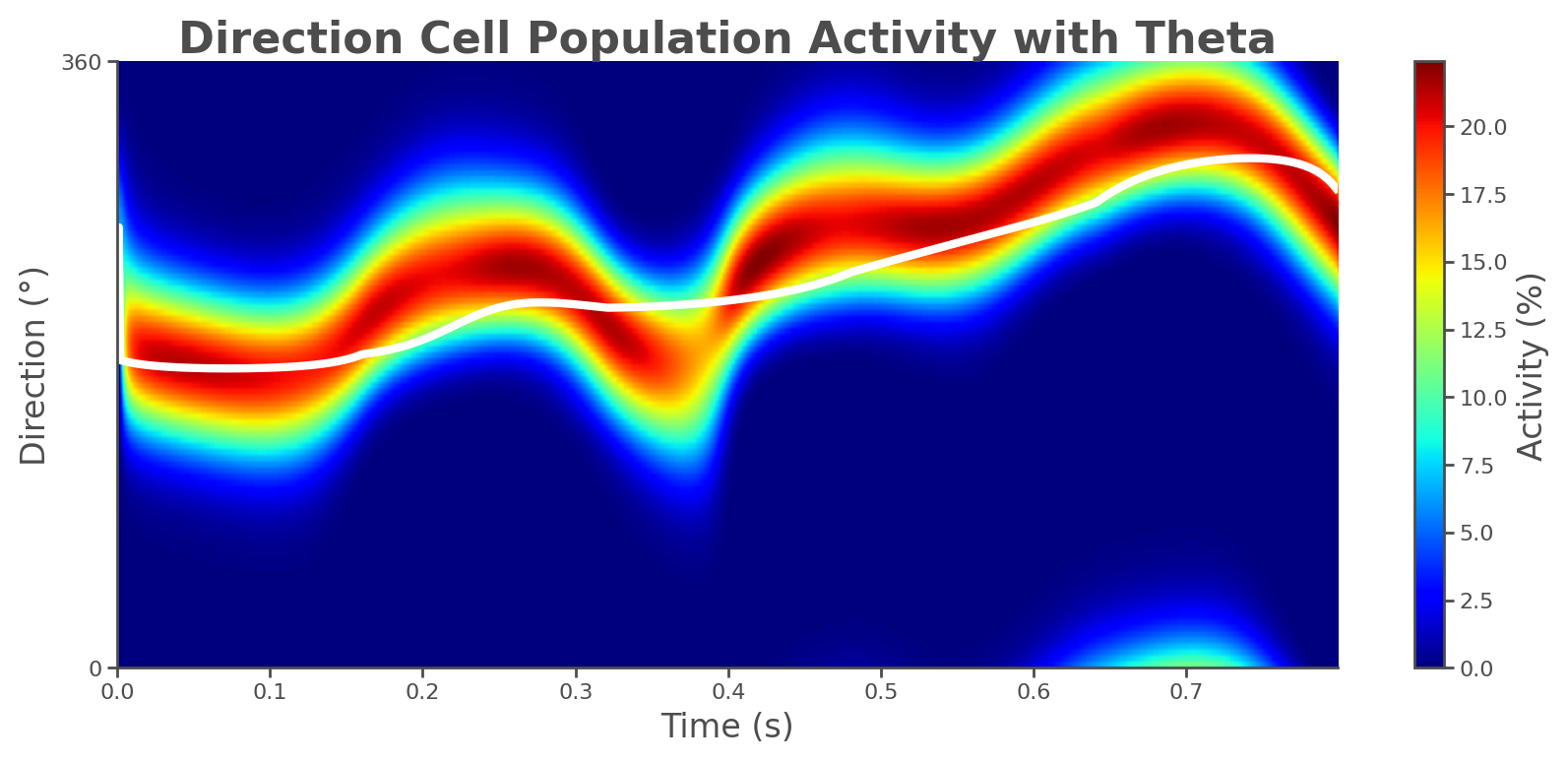
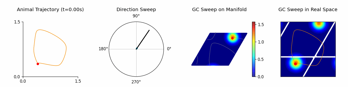
The returned results dictionary contains the animation, trajectory analysis, and raw simulation data, which can feed follow-up analyses.

Extension Guidelines

To customise a pipeline:

• Inherit canns.pipeline.Pipeline and implement run(...), returning a dictionary of primary artefacts.

• Call prepare_output_dir() as needed and cache outputs with set_results() for later use via get_results().

• Orchestrate models, tasks, and analyzers inside run() while keeping input and output formats explicit.

• Invoke reset() before repeated executions to clear cached state.