CANNs 介绍
![]()
![]()
欢迎使用 CANNs(连续吸引子神经网络)库!本笔记本介绍了这一强大神经网络建模框架的关键概念和功能。
什么是连续吸引子神经网络?
连续吸引子神经网络(CANNs)是一类特殊的神经网络模型,能够在连续状态空间中维持稳定的活动模式。与传统的处理离散输入输出的神经网络不同,CANNs 在以下方面表现优异:
空间表示:通过群体活动编码连续的空间位置
工作记忆:随时间维持和更新动态信息
路径积分:基于运动信息计算位置变化
平滑跟踪:跟踪连续变化的目标
CANNs 库的关键特性
🏗️ 丰富的模型库
CANN1D/2D:一维和二维连续吸引子网络
SFA 模型:集成慢特征分析的模型
分层网络:用于复杂信息处理的多层架构
🎮 面向任务的设计
路径积分:空间导航和位置估计任务
目标跟踪:动态目标的平滑连续跟踪
可扩展框架:轻松添加自定义任务类型
📊 强大的分析工具
实时可视化:能量景观、神经活动动画
统计分析:放电率、调谐曲线、群体动态
数据处理:z-score 标准化、时间序列分析
⚡ 高性能计算
JAX 加速:基于 JAX 的高效数值计算
GPU 支持:CUDA 和 TPU 硬件加速
并行处理:针对大规模网络仿真进行优化
安装
CANNs 库可以使用 pip 安装,并根据您的硬件配置不同的版本:
[ ]:
# 安装 CANNs(在终端中运行,不是在 notebook 中)
# 基础安装(CPU)
# !pip install canns

# GPU 支持(Linux)
# !pip install canns[cuda12]

# TPU 支持(Linux)
# !pip install canns[tpu]
基本使用示例
让我们从一个简单的示例开始,演示 CANNs 库的基本用法:
首先设置matplotlib的中文字体支持:
[5]:
import brainstate
from canns.models.basic import CANN1D
from canns.task.tracking import SmoothTracking1D
from canns.analyzer.visualize import energy_landscape_1d_animation, energy_landscape_1d_static
import numpy as np

# 设置计算环境
brainstate.environ.set(dt=0.1)
print("BrainState environment configured with dt=0.1")
BrainState environment configured with dt=0.1
[6]:
# 创建一个 1D CANN 网络
cann = CANN1D(num=512)
cann.init_state()

print(f"Created CANN1D with {cann.shape[0]} neurons")
print(f"Network shape: {cann.shape}")
print(f"Feature space range: [{cann.x.min():.2f}, {cann.x.max():.2f}]")
Created CANN1D with 512 neurons
Network shape: (512,)
Feature space range: [-3.14, 3.14]
了解网络结构
让我们探索 CANN 网络的基本属性:
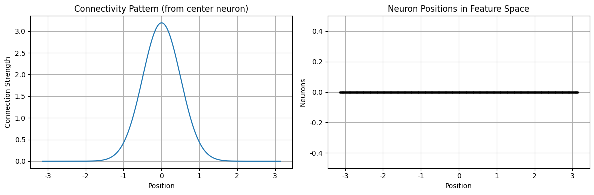
[7]:
# 检查连接矩阵
import matplotlib.pyplot as plt

# 绘制连接矩阵(可视化的一小部分)
fig, (ax1, ax2) = plt.subplots(1, 2, figsize=(12, 4))

# 绘制连接模式
center_idx = cann.shape[0] // 2
connectivity_slice = cann.conn_mat[center_idx, :]
ax1.plot(cann.x, connectivity_slice)
ax1.set_title('Connectivity Pattern (from center neuron)')
ax1.set_xlabel('Position')
ax1.set_ylabel('Connection Strength')
ax1.grid(True)

# 绘制网络位置
ax2.plot(cann.x, np.zeros_like(cann.x), 'ko', markersize=2)
ax2.set_title('Neuron Positions in Feature Space')
ax2.set_xlabel('Position')
ax2.set_ylabel('Neurons')
ax2.set_ylim(-0.5, 0.5)
ax2.grid(True)

plt.tight_layout()
plt.show()
创建简单跟踪任务
现在让我们创建一个平滑跟踪任务来观察网络的运行:
[8]:
# 定义平滑跟踪任务
task = SmoothTracking1D(
    cann_instance=cann,
    Iext=(1., 0.75, 2., 1.75, 3.),  # 外部输入序列
    duration=(10., 10., 10., 10.),   # 每个阶段的持续时间
    time_step=brainstate.environ.get_dt(),
)

# 获取任务数据
task.get_data()

print(f"Task created with {len(task.data)} time steps")
print(f"Input sequence: {task.Iext}")
print(f"Phase durations: {task.duration}")
<SmoothTracking1D> Generating Task data: 400it [00:00, 2535.27it/s]
Task created with 400 time steps
Input sequence: (1.0, 0.75, 2.0, 1.75, 3.0)
Phase durations: (10.0, 10.0, 10.0, 10.0)
运行仿真
让我们运行网络仿真并观察其行为:
[9]:
# 定义仿真步骤
def run_step(t, inputs):
    cann(inputs)
    return cann.u.value, cann.inp.value

# 运行仿真
print("Running simulation...")
us, inps = brainstate.compile.for_loop(
    run_step,
    task.run_steps,
    task.data,
    pbar=brainstate.compile.ProgressBar(10)
)

print(f"Simulation completed!")
print(f"Output shape: {us.shape}")
print(f"Input shape: {inps.shape}")
/Users/sichaohe/Documents/GitHub/canns/.venv/lib/python3.12/site-packages/tqdm/auto.py:21: TqdmWarning: IProgress not found. Please update jupyter and ipywidgets. See https://ipywidgets.readthedocs.io/en/stable/user_install.html
  from .autonotebook import tqdm as notebook_tqdm
Running simulation...
Running for 400 iterations: 100%|██████████| 400/400 [00:00<00:00, 57878.41it/s]
Simulation completed!
Output shape: (400, 512)
Input shape: (400, 512)
可视化结果
现在让我们可视化网络活动,看看它是如何跟踪输入的:
[10]:
# 创建能量景观动画
print("Generating energy landscape animation...")
energy_landscape_1d_animation(
    {'u': (cann.x, us), 'Iext': (cann.x, inps)},
    time_steps_per_second=50,
    fps=10,
    title='1D CANN Smooth Tracking Demo',
    xlabel='Position',
    ylabel='Activity',
    save_path='introduction_demo.gif',
    show=True,
)
print("Animation saved as 'introduction_demo.gif'")
Generating energy landscape animation...
<energy_landscape_1d_animation> Saving to introduction_demo.gif: 100%|██████████| 80/80 [00:04<00:00, 18.87it/s]
Animation successfully saved to: introduction_demo.gif
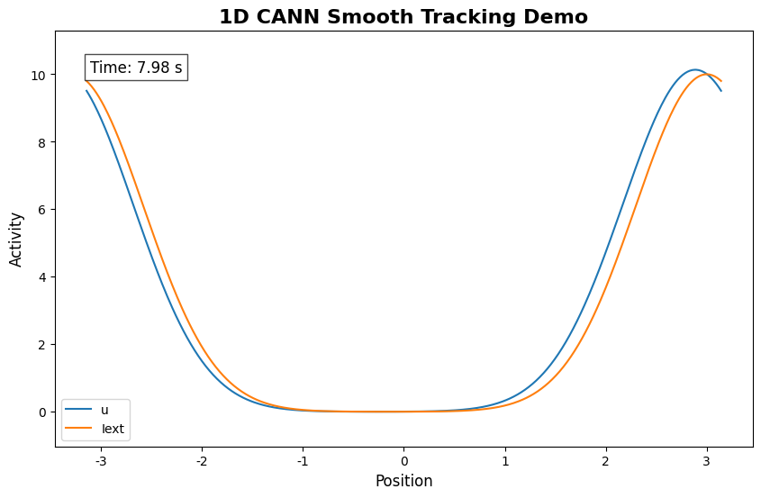
Animation saved as 'introduction_demo.gif'
关键观察结果
从这个基本示例中,您应该观察到:
平滑跟踪:网络活动(蓝线)平滑地跟随外部输入(红色虚线)
连续表示:活动形成一个在特征空间中连续移动的平滑波包
稳定动态:即使在输入变化时,网络也能维持稳定的活动模式
群体编码:多个神经元共同参与表示每个位置
下一步
本介绍涵盖了 CANNs 库的基础知识。在接下来的笔记本中,您将学习:
核心概念:深入了解数学基础
1D 网络:一维 CANNs 的详细探索
2D 网络:二维空间表示
分层模型:多层架构
自定义任务:创建您自己的任务和实验
可视化:高级绘图和分析技术
性能:大规模仿真的优化和扩展
资源
GitHub 仓库:https://github.com/routhleck/canns
文档:ReadTheDocs
示例:查看仓库中的
examples/目录
准备探索更多内容?让我们继续学习核心概念!