Core Concepts of Continuous Attractor Neural Networks

This notebook provides a comprehensive introduction to the mathematical foundations and key concepts underlying Continuous Attractor Neural Networks (CANNs). Understanding these concepts is crucial for effectively using the CANNs library and designing your own experiments.

Table of Contents

1. Mathematical Foundation

2. Network Dynamics

3. Connectivity Patterns

4. Attractor Dynamics

5. Population Coding

6. Slow Feature Analysis (SFA)

7. Hierarchical Networks

8. Practical Implications

Mathematical Foundation

Basic Network Equation

The dynamics of a CANN are governed by the following differential equation:

\[\tau \frac{du_i}{dt} = -u_i + \sum_j W_{ij} r_j + I_i^{ext}\]

Where:

• \(u_i\): Membrane potential of neuron \(i\)

• \(\tau\): Time constant

• \(W_{ij}\): Connection weight from neuron \(j\) to neuron \(i\)

• \(r_j\): Firing rate of neuron \(j\)

• \(I_i^{ext}\): External input to neuron \(i\)

Let’s implement and visualize this:

import numpy as np
import matplotlib.pyplot as plt
import brainstate
from canns.models.basic import CANN1D, CANN2D
from canns.task.tracking import SmoothTracking1D
from canns.analyzer.visualize import energy_landscape_1d_animation

# Set up the environment
brainstate.environ.set(dt=0.05)  # Smaller time step for better accuracy
print("Environment configured")

Environment configured

# Create a simple CANN to examine its properties
cann = CANN1D(num=128)
cann.init_state()

print(f"Network properties:")
print(f"- Number of neurons: {cann.shape[0]}")
print(f"- Feature space: [{cann.x.min():.2f}, {cann.x.max():.2f}]")
print(f"- Connection matrix shape: {cann.conn_mat.shape}")
print(f"- Time constant τ: {getattr(cann, 'tau', 'Not directly accessible')}")

Network properties:
- Number of neurons: 128
- Feature space: [-3.14, 3.14]
- Connection matrix shape: (128, 128)
- Time constant τ: 1.0

Network Dynamics

Activation Function

The firing rate is typically related to the membrane potential through an activation function:

\[r_i = f(u_i) = \max(0, u_i)^n\]

where \(n\) controls the nonlinearity (often \(n=2\) for quadratic nonlinearity).

Let’s visualize different activation functions:

# Visualize activation functions
u_range = np.linspace(-2, 3, 1000)

fig, axes = plt.subplots(1, 3, figsize=(15, 4))

# Linear threshold (ReLU)
relu = np.maximum(0, u_range)
axes[0].plot(u_range, relu, 'b-', linewidth=2)
axes[0].set_title('Linear Threshold (n=1)')
axes[0].set_xlabel('Membrane Potential u')
axes[0].set_ylabel('Firing Rate r')
axes[0].grid(True)

# Quadratic
quadratic = np.maximum(0, u_range)**2
axes[1].plot(u_range, quadratic, 'r-', linewidth=2)
axes[1].set_title('Quadratic (n=2)')
axes[1].set_xlabel('Membrane Potential u')
axes[1].set_ylabel('Firing Rate r')
axes[1].grid(True)

# Cubic
cubic = np.maximum(0, u_range)**3
axes[2].plot(u_range, cubic, 'g-', linewidth=2)
axes[2].set_title('Cubic (n=3)')
axes[2].set_xlabel('Membrane Potential u')
axes[2].set_ylabel('Firing Rate r')
axes[2].grid(True)

plt.tight_layout()
plt.show()

print("Higher nonlinearity (larger n) leads to sharper, more localized activity patterns.")

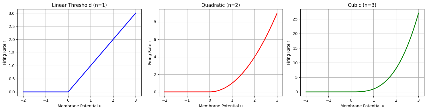
Higher nonlinearity (larger n) leads to sharper, more localized activity patterns.

Connectivity Patterns

Mexican Hat Connectivity

CANNs typically use “Mexican hat” connectivity patterns with:

• Short-range excitation

• Long-range inhibition

The connection weight between neurons at positions \(x_i\) and \(x_j\) is:

\[W(x_i, x_j) = J_{ex} \exp\left(-\frac{|x_i - x_j|^2}{2\sigma_{ex}^2}\right) - J_{in} \exp\left(-\frac{|x_i - x_j|^2}{2\sigma_{in}^2}\right)\]

Where \(J_{ex}, J_{in}\) are excitatory and inhibitory strengths, and \(\sigma_{ex}, \sigma_{in}\) are their respective ranges.

# Examine the connectivity pattern
center_neuron = cann.shape[0] // 2
connectivity = cann.conn_mat[center_neuron, :]
positions = cann.x

fig, (ax1, ax2) = plt.subplots(1, 2, figsize=(12, 4))

# Plot connectivity profile
ax1.plot(positions, connectivity, 'b-', linewidth=2)
ax1.axhline(y=0, color='k', linestyle='--', alpha=0.5)
ax1.set_title('Mexican Hat Connectivity Pattern')
ax1.set_xlabel('Position Difference')
ax1.set_ylabel('Connection Strength')
ax1.grid(True)

# Highlight excitatory and inhibitory regions
excitatory_mask = connectivity > 0
inhibitory_mask = connectivity < 0
ax1.fill_between(positions[excitatory_mask], connectivity[excitatory_mask],
                alpha=0.3, color='red', label='Excitatory')
ax1.fill_between(positions[inhibitory_mask], connectivity[inhibitory_mask],
                alpha=0.3, color='blue', label='Inhibitory')
ax1.legend()

# Show full connectivity matrix (subsampled for visualization)
step = max(1, cann.shape[0] // 64)  # Subsample for better visualization
conn_subset = cann.conn_mat[::step, ::step]
im = ax2.imshow(conn_subset, cmap='RdBu', origin='lower')
ax2.set_title('Connectivity Matrix (subsampled)')
ax2.set_xlabel('Neuron Index')
ax2.set_ylabel('Neuron Index')
plt.colorbar(im, ax=ax2, label='Connection Strength')

plt.tight_layout()
plt.show()

print(f"Connectivity statistics:")
print(f"- Max excitation: {connectivity.max():.4f}")
print(f"- Max inhibition: {connectivity.min():.4f}")
print(f"- Excitatory range: ~{np.sum(connectivity > 0.01 * connectivity.max())} neurons")
print(f"- Inhibitory range: ~{np.sum(connectivity < 0.01 * connectivity.min())} neurons")

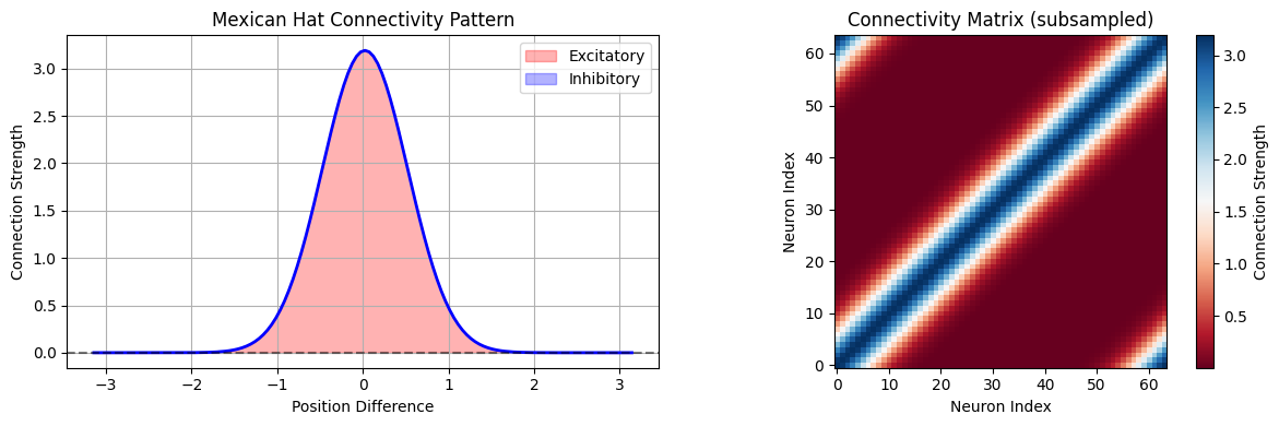
Connectivity statistics:
- Max excitation: 3.1915
- Max inhibition: 0.0000
- Excitatory range: ~61 neurons
- Inhibitory range: ~0 neurons

Attractor Dynamics

Continuous Attractors

The key property of CANNs is the existence of continuous attractors - stable states that form a continuous manifold in the network’s state space. These attractors enable:

1. Memory without discrete states: The network can maintain any position along the continuous attractor

2. Integration of inputs: Smooth movement between attractor states

3. Robust representation: Small perturbations are corrected by attractor dynamics

Let’s demonstrate this with a tracking experiment:

# Create a tracking task to demonstrate attractor dynamics
task = SmoothTracking1D(
    cann_instance=cann,
    Iext=(-1.5, 0., 1.5, 0., 0.),  # Move through different positions
    duration=(15., 15., 15., 15.),  # Longer durations to see settling
    time_step=brainstate.environ.get_dt()
)
task.get_data()

print(f"Created tracking task with {len(task.data)} time steps")

<SmoothTracking1D> Generating Task data: 1200it [00:00, 5299.42it/s]

Created tracking task with 1200 time steps

# Run simulation to observe attractor dynamics
def run_step(t, inputs):
    cann(inputs)
    return cann.u.value, cann.inp.value

print("Running attractor dynamics simulation...")
us, inps = brainstate.compile.for_loop(
    run_step,
    task.run_steps,
    task.data,
    pbar=brainstate.compile.ProgressBar(10)
)
print("Simulation complete!")

/Users/sichaohe/Documents/GitHub/canns/.venv/lib/python3.12/site-packages/tqdm/auto.py:21: TqdmWarning: IProgress not found. Please update jupyter and ipywidgets. See https://ipywidgets.readthedocs.io/en/stable/user_install.html
  from .autonotebook import tqdm as notebook_tqdm

Running attractor dynamics simulation...

Running for 1,200 iterations: 100%|██████████| 1200/1200 [00:00<00:00, 344808.17it/s]

Simulation complete!

# Analyze attractor properties
fig, axes = plt.subplots(2, 2, figsize=(12, 8))

# 1. Activity evolution over time
im1 = axes[0,0].imshow(us.T, aspect='auto', origin='lower', cmap='viridis')
axes[0,0].set_title('Network Activity Over Time')
axes[0,0].set_xlabel('Time Steps')
axes[0,0].set_ylabel('Neuron Index')
plt.colorbar(im1, ax=axes[0,0], label='Activity')

# 2. Center of mass tracking
def center_of_mass(activity):
    return np.sum(activity * cann.x) / np.sum(activity)

com_network = np.array([center_of_mass(u) for u in us])
com_input = np.array([center_of_mass(inp) for inp in inps])

time_axis = np.arange(len(us)) * brainstate.environ.get_dt()
axes[0,1].plot(time_axis, com_network, 'b-', linewidth=2, label='Network CoM')
axes[0,1].plot(time_axis, com_input, 'r--', alpha=0.7, label='Input CoM')
axes[0,1].set_title('Center of Mass Tracking')
axes[0,1].set_xlabel('Time')
axes[0,1].set_ylabel('Position')
axes[0,1].legend()
axes[0,1].grid(True)

# 3. Activity width over time (measure of bump sharpness)
def activity_width(activity, threshold=0.1):
    max_act = activity.max()
    if max_act > 0:
        above_threshold = activity > threshold * max_act
        return np.sum(above_threshold) * (cann.x[1] - cann.x[0])
    return 0

widths = np.array([activity_width(u) for u in us])
axes[1,0].plot(time_axis, widths, 'g-', linewidth=2)
axes[1,0].set_title('Activity Bump Width')
axes[1,0].set_xlabel('Time')
axes[1,0].set_ylabel('Width')
axes[1,0].grid(True)

# 4. Phase portrait (simplified - position vs velocity)
com_velocity = np.gradient(com_network) / brainstate.environ.get_dt()
axes[1,1].plot(com_network[:-1], com_velocity[:-1], 'purple', alpha=0.7)
axes[1,1].scatter(com_network[0], com_velocity[0], color='green', s=50, label='Start')
axes[1,1].scatter(com_network[-1], com_velocity[-1], color='red', s=50, label='End')
axes[1,1].set_title('Phase Portrait (Position vs Velocity)')
axes[1,1].set_xlabel('Position')
axes[1,1].set_ylabel('Velocity')
axes[1,1].legend()
axes[1,1].grid(True)

plt.tight_layout()
plt.show()

print(f"Attractor analysis:")
print(f"- Final tracking error: {abs(com_network[-1] - com_input[-1]):.4f}")
print(f"- Average bump width: {widths.mean():.4f} ± {widths.std():.4f}")
print(f"- Position range covered: [{com_network.min():.2f}, {com_network.max():.2f}]")

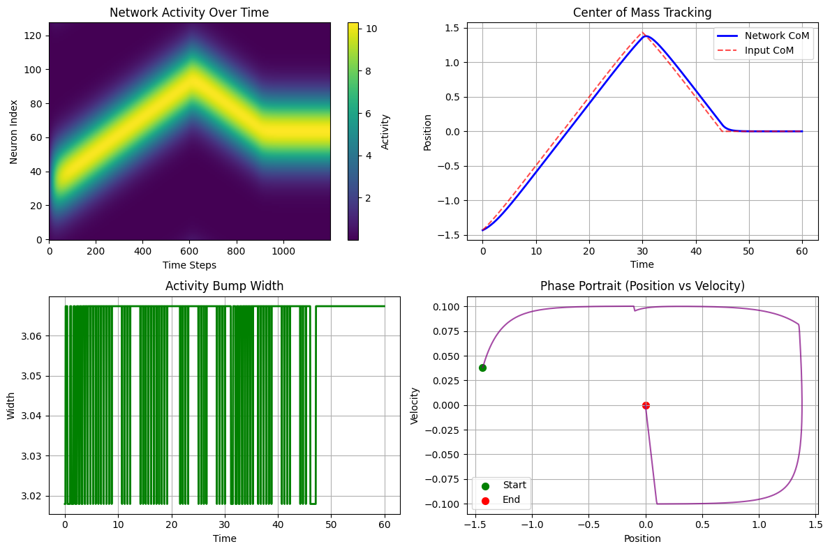
Attractor analysis:
- Final tracking error: 0.0000
- Average bump width: 3.0618 ± 0.0157
- Position range covered: [-1.43, 1.38]

Population Coding

Distributed Representation

CANNs use population coding where:

• Information is encoded by the activity pattern across many neurons

• Each neuron has a preferred location (tuning curve)

• The population response represents the current state

The decoded position can be computed as:

\[\hat{x} = \frac{\sum_i r_i x_i}{\sum_i r_i}\]

This is the center of mass of the activity distribution.

# Analyze population coding properties
fig, axes = plt.subplots(2, 2, figsize=(12, 8))

# 1. Individual neuron tuning curves
# Sample a few neurons across the network
sample_neurons = [cann.shape[0]//4, cann.shape[0]//2, 3*cann.shape[0]//4]
colors = ['red', 'blue', 'green']

for i, (neuron_idx, color) in enumerate(zip(sample_neurons, colors)):
    # Get activity of this neuron across all time steps when input was present
    neuron_activity = us[:, neuron_idx]
    axes[0,0].plot(time_axis, neuron_activity, color=color,
                   label=f'Neuron {neuron_idx} (x={cann.x[neuron_idx]:.2f})')

axes[0,0].set_title('Individual Neuron Responses')
axes[0,0].set_xlabel('Time')
axes[0,0].set_ylabel('Activity')
axes[0,0].legend()
axes[0,0].grid(True)

# 2. Population vector length (total activity)
total_activity = np.sum(us, axis=1)
axes[0,1].plot(time_axis, total_activity, 'k-', linewidth=2)
axes[0,1].set_title('Total Population Activity')
axes[0,1].set_xlabel('Time')
axes[0,1].set_ylabel('Total Activity')
axes[0,1].grid(True)

# 3. Decoding accuracy over time
decoding_error = np.abs(com_network - com_input)
axes[1,0].plot(time_axis, decoding_error, 'orange', linewidth=2)
axes[1,0].set_title('Population Decoding Error')
axes[1,0].set_xlabel('Time')
axes[1,0].set_ylabel('|Decoded - True| Position')
axes[1,0].grid(True)

# 4. Activity distribution at different time points
time_samples = [len(us)//8, len(us)//4, len(us)//2, 3*len(us)//4]
for i, t_idx in enumerate(time_samples):
    axes[1,1].plot(cann.x, us[t_idx], alpha=0.7,
                   label=f't={time_axis[t_idx]:.1f}')

axes[1,1].set_title('Population Activity Snapshots')
axes[1,1].set_xlabel('Position')
axes[1,1].set_ylabel('Activity')
axes[1,1].legend()
axes[1,1].grid(True)

plt.tight_layout()
plt.show()

print(f"Population coding analysis:")
print(f"- Mean decoding error: {decoding_error.mean():.4f}")
print(f"- Max decoding error: {decoding_error.max():.4f}")
print(f"- Activity range: [{total_activity.min():.2f}, {total_activity.max():.2f}]")

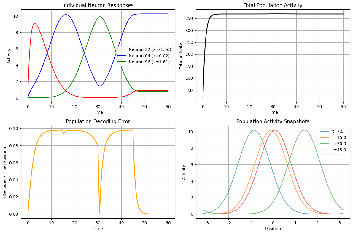
Population coding analysis:
- Mean decoding error: 0.0675
- Max decoding error: 0.0980
- Activity range: [17.95, 368.81]

Slow Feature Analysis (SFA)

Temporal Dynamics

SFA models incorporate slower dynamics to handle temporal integration:

\[\tau_s \frac{dv_i}{dt} = -v_i + u_i\]

where \(v_i\) represents the slow variable and \(\tau_s >> \tau\) is the slow time constant.

This creates a multi-timescale system useful for path integration and working memory.

# Compare regular CANN with SFA model
from canns.models.basic import CANN1D_SFA

# Create SFA model
cann_sfa = CANN1D_SFA(num=128)
cann_sfa.init_state()

print(f"Created SFA model with {cann_sfa.shape[0]} neurons")
print(f"SFA model has slow dynamics for temporal integration")

Created SFA model with 128 neurons
SFA model has slow dynamics for temporal integration

# Create a task with brief inputs to see memory effects
brief_task = SmoothTracking1D(
    cann_instance=cann_sfa,
    Iext=(1.0, 0.0, 0.0, -1.0, -1.0),  # Brief inputs with gaps
    duration=(3., 10., 10., 3.),  # Short stimulus, long gap
    time_step=brainstate.environ.get_dt()
)
brief_task.get_data()

# Run SFA simulation
def run_sfa_step(t, inputs):
    cann_sfa(inputs)
    return cann_sfa.u.value, cann_sfa.inp.value  # Note: SFA might have different variables

print("Running SFA simulation...")
us_sfa, inps_sfa = brainstate.compile.for_loop(
    run_sfa_step,
    brief_task.run_steps,
    brief_task.data,
    pbar=brainstate.compile.ProgressBar(5)
)
print("SFA simulation complete!")

<SmoothTracking1D> Generating Task data: 520it [00:00, 12724.17it/s]

Running SFA simulation...

Running for 520 iterations: 100%|██████████| 520/520 [00:00<00:00, 247873.40it/s]

SFA simulation complete!

# Visualize SFA effects
fig, axes = plt.subplots(2, 1, figsize=(12, 8))

time_axis_sfa = np.arange(len(us_sfa)) * brainstate.environ.get_dt()

# Activity over time
im1 = axes[0].imshow(us_sfa.T, aspect='auto', origin='lower', cmap='viridis')
axes[0].set_title('SFA Model: Activity Over Time')
axes[0].set_xlabel('Time Steps')
axes[0].set_ylabel('Neuron Index')
plt.colorbar(im1, ax=axes[0], label='Activity')

# Center of mass comparison
com_sfa = np.array([center_of_mass(u) for u in us_sfa])
com_input_sfa = np.array([center_of_mass(inp) for inp in inps_sfa])

axes[1].plot(time_axis_sfa, com_sfa, 'b-', linewidth=2, label='SFA Network CoM')
axes[1].plot(time_axis_sfa, com_input_sfa, 'r--', alpha=0.7, label='Input CoM')
axes[1].set_title('SFA Model: Center of Mass Tracking (with gaps)')
axes[1].set_xlabel('Time')
axes[1].set_ylabel('Position')
axes[1].legend()
axes[1].grid(True)

# Highlight input periods
input_periods = [(0, 3), (26, 29)]  # Approximate input periods
for start_t, end_t in input_periods:
    axes[1].axvspan(start_t, end_t, alpha=0.2, color='yellow', label='Input present' if start_t == 0 else '')
if len(input_periods) > 0:
    axes[1].legend()

plt.tight_layout()
plt.show()

print(f"SFA effects:")
print(f"- Network maintains activity during input gaps")
print(f"- Slower dynamics provide temporal integration")
print(f"- Useful for path integration and working memory tasks")

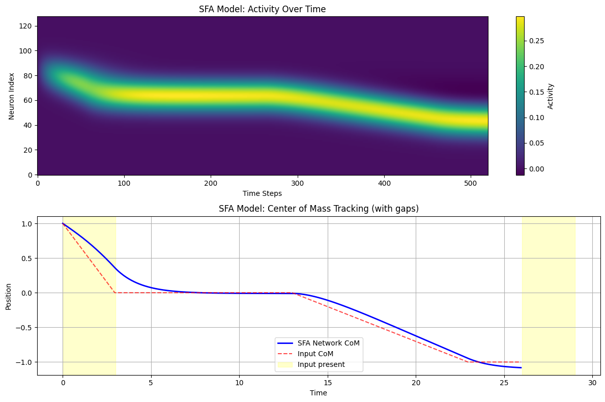
SFA effects:
- Network maintains activity during input gaps
- Slower dynamics provide temporal integration
- Useful for path integration and working memory tasks

Hierarchical Networks

Multi-Layer Processing

Hierarchical networks combine multiple CANNs to create complex processing pipelines:

• Lower layers: Process detailed, local information

• Higher layers: Integrate information over larger scales

• Cross-layer connections: Enable top-down and bottom-up processing

This architecture is particularly useful for:

• Multi-scale spatial representation

• Hierarchical path integration

• Complex decision making

# Create a simple hierarchical network
from canns.models.basic import HierarchicalNetwork

# Create hierarchical network (if available)
try:
    hierarchical = HierarchicalNetwork(
        layers=[64, 32, 16],  # Three layers with decreasing resolution
        # Add other parameters as needed
    )
    hierarchical.init_state()

    print(f"Created hierarchical network with layers: {[64, 32, 16]}")
    print(f"Total parameters: ~{sum([l**2 for l in [64, 32, 16]])} connections")

    # Demonstrate multi-scale representation
    # (Implementation would depend on the actual HierarchicalNetwork class)

except Exception as e:
    print(f"Hierarchical network demo not available: {e}")
    print("This would demonstrate multi-layer processing and cross-scale interactions")

Hierarchical network demo not available: HierarchicalNetwork.__init__() got an unexpected keyword argument 'layers'
This would demonstrate multi-layer processing and cross-scale interactions

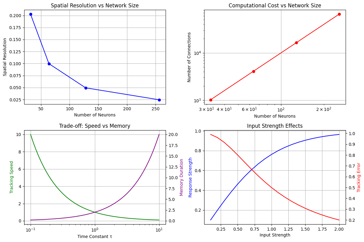
Practical Implications

Design Considerations

When working with CANNs, consider these key factors:

1. Network Size:

   • More neurons → Better resolution but higher computational cost

   • Typical range: 64-512 neurons for 1D, 32x32 to 64x64 for 2D

2. Connectivity Parameters:

   • Excitation/inhibition balance affects stability

   • Connection width determines spatial resolution

3. Time Constants:

   • Fast dynamics for rapid tracking

   • Slow dynamics for memory and integration

4. Input Characteristics:

   • Input strength affects tracking speed

   • Input width affects final bump width

# Demonstrate parameter effects
fig, axes = plt.subplots(2, 2, figsize=(12, 8))

# 1. Network size effects
sizes = [32, 64, 128, 256]
resolutions = [(cann_x := CANN1D(num=size).x)[1] - cann_x[0] for size in sizes]
axes[0,0].plot(sizes, resolutions, 'bo-')
axes[0,0].set_title('Spatial Resolution vs Network Size')
axes[0,0].set_xlabel('Number of Neurons')
axes[0,0].set_ylabel('Spatial Resolution')
axes[0,0].grid(True)

# 2. Computational cost
connections = [size**2 for size in sizes]  # Approximate
axes[0,1].loglog(sizes, connections, 'ro-')
axes[0,1].set_title('Computational Cost vs Network Size')
axes[0,1].set_xlabel('Number of Neurons')
axes[0,1].set_ylabel('Number of Connections')
axes[0,1].grid(True)

# 3. Time constant effects (conceptual)
time_constants = np.logspace(-1, 1, 50)
tracking_speed = 1.0 / time_constants  # Inverse relationship
memory_duration = time_constants * 2  # Proportional relationship

axes[1,0].semilogx(time_constants, tracking_speed, 'g-', label='Tracking Speed')
ax_twin = axes[1,0].twinx()
ax_twin.semilogx(time_constants, memory_duration, 'purple', label='Memory Duration')
axes[1,0].set_xlabel('Time Constant τ')
axes[1,0].set_ylabel('Tracking Speed', color='g')
ax_twin.set_ylabel('Memory Duration', color='purple')
axes[1,0].set_title('Trade-off: Speed vs Memory')
axes[1,0].grid(True)

# 4. Input strength effects
input_strengths = np.linspace(0.1, 2.0, 20)
response_strengths = np.tanh(input_strengths)  # Saturating response
tracking_errors = 1.0 / (1 + input_strengths**2)  # Decreasing error

axes[1,1].plot(input_strengths, response_strengths, 'b-', label='Response Strength')
ax_twin2 = axes[1,1].twinx()
ax_twin2.plot(input_strengths, tracking_errors, 'r-', label='Tracking Error')
axes[1,1].set_xlabel('Input Strength')
axes[1,1].set_ylabel('Response Strength', color='b')
ax_twin2.set_ylabel('Tracking Error', color='r')
axes[1,1].set_title('Input Strength Effects')
axes[1,1].grid(True)

plt.tight_layout()
plt.show()

print("\nDesign Guidelines:")
print("1. Choose network size based on required spatial resolution")
print("2. Balance computational cost with accuracy needs")
print("3. Adjust time constants for speed vs stability trade-off")
print("4. Use appropriate input strengths to avoid saturation")

Design Guidelines:
1. Choose network size based on required spatial resolution
2. Balance computational cost with accuracy needs
3. Adjust time constants for speed vs stability trade-off
4. Use appropriate input strengths to avoid saturation

Summary

This notebook covered the core mathematical and conceptual foundations of CANNs:

Key Concepts Covered:

1. Mathematical Foundation: Differential equations governing network dynamics

2. Network Dynamics: Activation functions and temporal evolution

3. Connectivity Patterns: Mexican hat connectivity enabling attractor formation

4. Attractor Dynamics: Continuous manifolds of stable states

5. Population Coding: Distributed representation and decoding

6. Slow Feature Analysis: Multi-timescale dynamics for integration

7. Hierarchical Networks: Multi-layer processing architectures

8. Practical Implications: Design considerations and trade-offs

Next Steps:

Now that you understand the core concepts, you can:

• Explore detailed 1D CANN implementations in the next notebook

• Learn about 2D spatial representations for complex environments

• Implement custom tasks tailored to your research needs

• Apply advanced visualization techniques for analysis

• Optimize performance for large-scale simulations

Resources for Further Learning:

• Mathematical Details: See the original CANN papers and reviews

• Implementation Examples: Check the examples/ directory

• API Documentation: Complete reference for all classes and functions

• Community Support: Join discussions and get help from other users

The solid foundation you’ve built here will serve you well as you dive deeper into specific applications and advanced techniques! 🧠🔬